exploration

Library

library(tidyverse) #For plotting and wrangling

── Attaching packages ─────────────────────────────────────── tidyverse 1.3.2 ──
✔ ggplot2 3.4.0     ✔ purrr   1.0.1
✔ tibble  3.1.8     ✔ dplyr   1.1.0
✔ tidyr   1.2.1     ✔ stringr 1.5.0
✔ readr   2.1.3     ✔ forcats 0.5.2
── Conflicts ────────────────────────────────────────── tidyverse_conflicts() ──
✖ dplyr::filter() masks stats::filter()
✖ dplyr::lag()    masks stats::lag()

library(here) #Setting working directory

here() starts at /Users/nathangreenslit/Desktop/UGA/Spring 2023/MADA/nathangreenslit-MADA-portfolio

library(gtsummary) #For summary tables

Load Data

d<- readRDS(here("fluanalysis", "data", "SypAct_clean.rds"))

Produce and Print a Summary Table for both Body Temperature and Nausea

Summary Stats

summary(d$BodyTemp)

   Min. 1st Qu.  Median    Mean 3rd Qu.    Max. 
  97.20   98.20   98.50   98.94   99.30  103.10

summary(d$Nausea)

 No Yes 
475 255

Summary of full data set

tab<- 
  tbl_summary(d)
tab

Characteristic	N = 730¹
Swollen Lymph Nodes	312 (43%)
Chest Congestion	407 (56%)
Chills/Sweats	600 (82%)
Nasal Congestion	563 (77%)
Sneeze	391 (54%)
Fatigue	666 (91%)
Subjective Fever	500 (68%)
Headache	615 (84%)
Weakness
None	49 (6.7%)
Mild	223 (31%)
Moderate	338 (46%)
Severe	120 (16%)
Cough Severity
None	47 (6.4%)
Mild	154 (21%)
Moderate	357 (49%)
Severe	172 (24%)
Myalgia
None	79 (11%)
Mild	213 (29%)
Moderate	325 (45%)
Severe	113 (15%)
Runny Nose	519 (71%)
Abdominal Pain	91 (12%)
Chest Pain	233 (32%)
Diarrhea	99 (14%)
Eye Pain	113 (15%)
Sleeplessness	415 (57%)
Itchy Eyes	179 (25%)
Nausea	255 (35%)
Ear Pain	162 (22%)
Sore Throat	611 (84%)
Breathlessness	294 (40%)
Tooth Pain	165 (23%)
Vomiting	78 (11%)
Wheezing	220 (30%)
BodyTemp	98.50 (98.20, 99.30)
¹ n (%); Median (IQR)

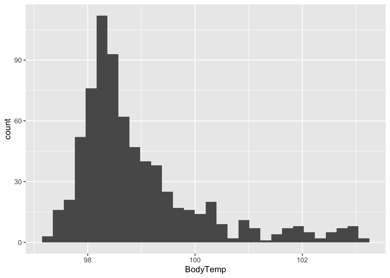
Create Histogram for Body Temperature

d %>%
  ggplot()+geom_histogram(
    aes(
      x = BodyTemp))

`stat_bin()` using `bins = 30`. Pick better value with `binwidth`.

A majority of the body temperatures fall between 98-99°F

Let’s look at Predictor Variables for our outcomes of interest (Body Temperature and Nausea)

Body Temperature

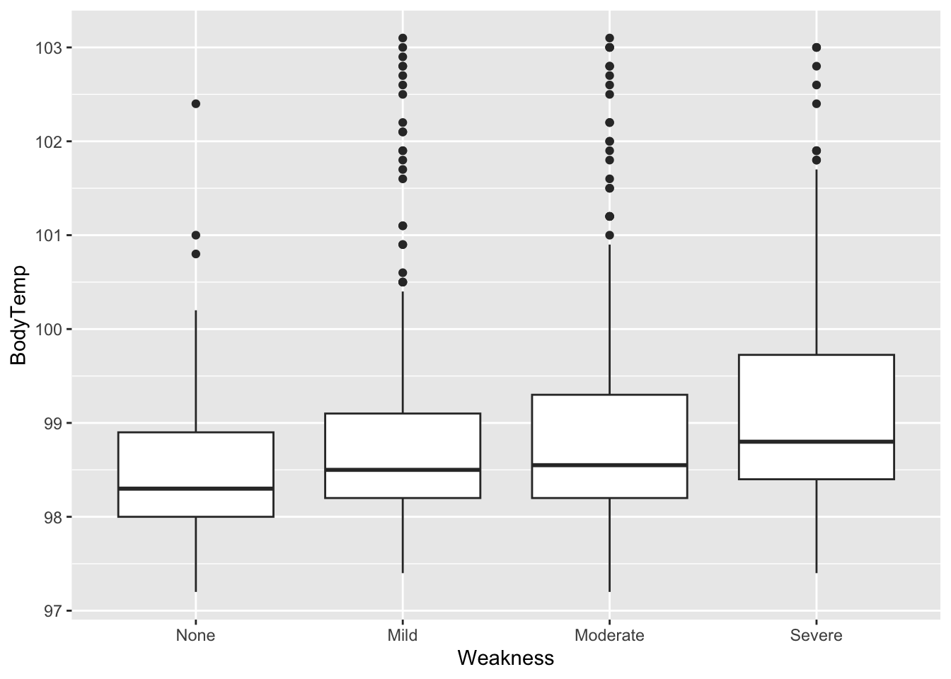
Weakness and Body Temp

d %>%
  ggplot()+geom_boxplot(
    aes(
      x= Weakness,
      y = BodyTemp))

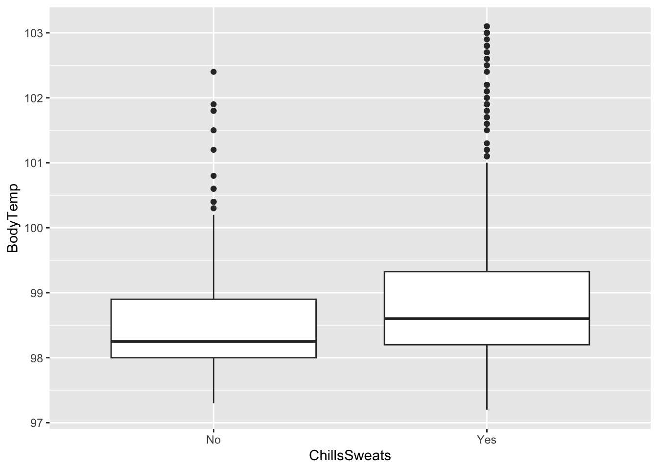
Chills and Sweats and Body Temp

d %>%
  ggplot()+geom_boxplot(
    aes(
      x= ChillsSweats,
      y = BodyTemp))

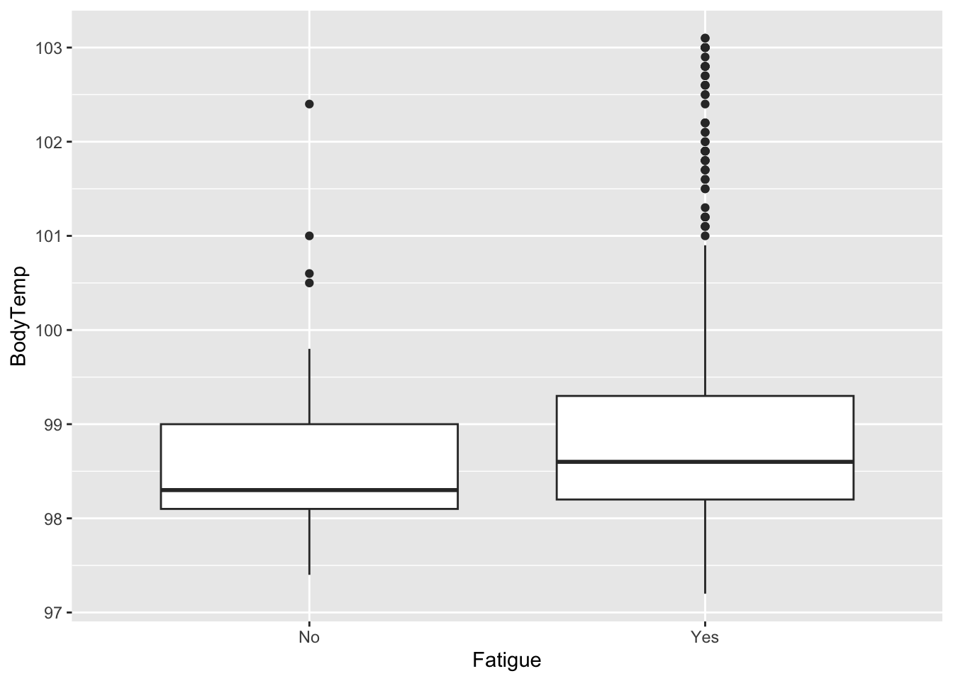
Fatigue and Body Temp

d %>%
  ggplot()+geom_boxplot(
    aes(
      x= Fatigue,
      y = BodyTemp))

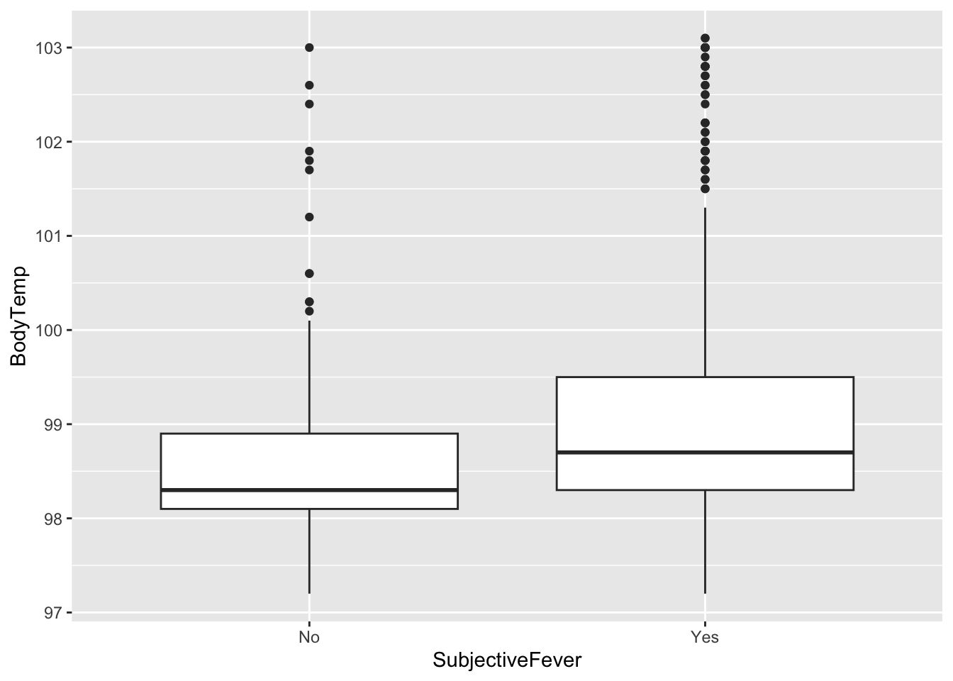
Fever and Body Temp

d %>%
  ggplot()+geom_boxplot(
    aes(
      x= SubjectiveFever,
      y = BodyTemp))

On average, it looks like those that experienced severe weakness symptoms, chills and sweats, fatigue, and fever had higher body temperatures. We would expect to see this positive relationship in the latter- so fever will be our main predictor of interest for Body Temperature.

Now let’s look at some predictor variables for the categorical variable (Nausea)

Diarrhea and Nausea

d %>%
  ggplot() + geom_count(
    aes(
      x = Nausea,
      y = Fatigue))

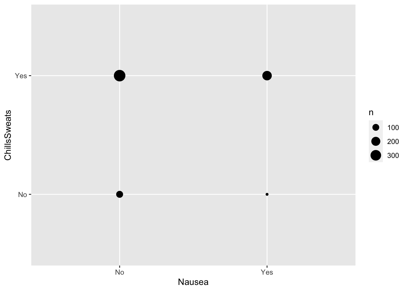
Chills and Nausea

d %>%
  ggplot() + geom_count(
    aes(
      x = Nausea,
      y = ChillsSweats))

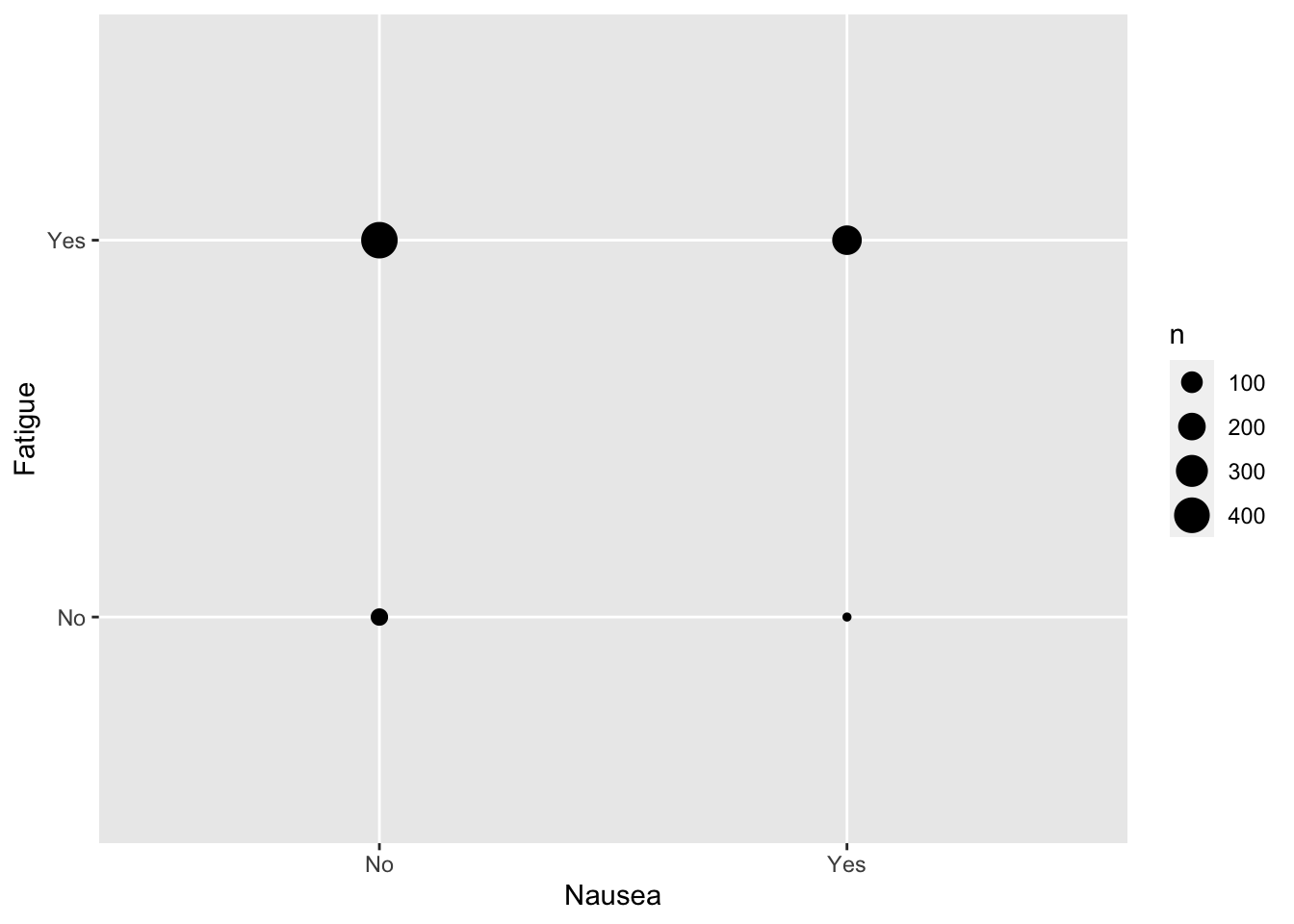
Fatigue and Nausea

d %>%
  ggplot() + geom_count(
    aes(
      x = Nausea,
      y = Fatigue))

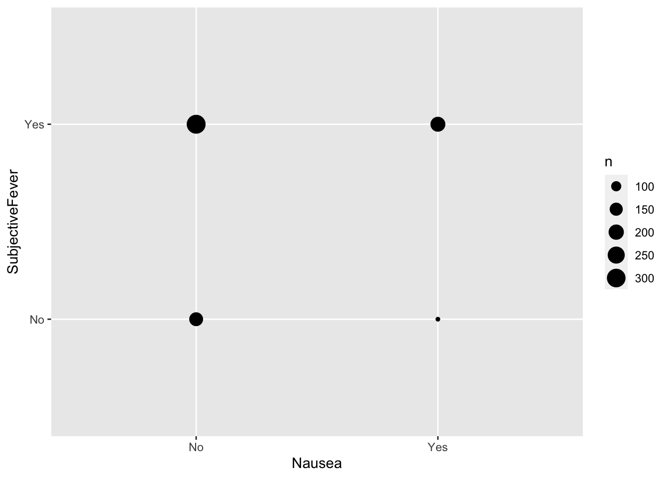
Fever and Nausea

d %>%
  ggplot() + geom_count(
    aes(
      x = Nausea,
      y = SubjectiveFever))

Fever, Fatigue, Chills, and Diarrhea all appear to have equal or no major positive relationship (Where x:nausea = Yes-Yes < Yes-No). Vomiting will be our predictor of interest for the categorical outcome (Nausea), as there was a large proportion that did not experience either Nausea or Vomiting, and a medium-proportion of those that experienced one symptom with the other.