Tidy Tuesday Exercise2

Getting Started

Libraries

library(tidyverse)

── Attaching packages ─────────────────────────────────────── tidyverse 1.3.2 ──
✔ ggplot2 3.4.0     ✔ purrr   1.0.1
✔ tibble  3.1.8     ✔ dplyr   1.1.0
✔ tidyr   1.2.1     ✔ stringr 1.5.0
✔ readr   2.1.3     ✔ forcats 0.5.2
── Conflicts ────────────────────────────────────────── tidyverse_conflicts() ──
✖ dplyr::filter() masks stats::filter()
✖ dplyr::lag()    masks stats::lag()

library(here)

here() starts at /Users/nathangreenslit/Desktop/UGA/Spring 2023/MADA/nathangreenslit-MADA-portfolio

library(rsample) #Data spliting
library(tidymodels)

── Attaching packages ────────────────────────────────────── tidymodels 1.0.0 ──
✔ broom        1.0.2     ✔ recipes      1.0.5
✔ dials        1.1.0     ✔ tune         1.0.1
✔ infer        1.0.4     ✔ workflows    1.1.3
✔ modeldata    1.1.0     ✔ workflowsets 1.0.0
✔ parsnip      1.0.4     ✔ yardstick    1.1.0
── Conflicts ───────────────────────────────────────── tidymodels_conflicts() ──
✖ scales::discard() masks purrr::discard()
✖ dplyr::filter()   masks stats::filter()
✖ recipes::fixed()  masks stringr::fixed()
✖ dplyr::lag()      masks stats::lag()
✖ yardstick::spec() masks readr::spec()
✖ recipes::step()   masks stats::step()
• Search for functions across packages at https://www.tidymodels.org/find/

tidymodels_prefer(quiet =FALSE) #Removes package masking conflicts

[conflicted] Will prefer dplyr::filter over any other package.
[conflicted] Will prefer dplyr::select over any other package.
[conflicted] Will prefer dplyr::slice over any other package.
[conflicted] Will prefer dplyr::rename over any other package.
[conflicted] Will prefer dials::neighbors over any other package.
[conflicted] Will prefer parsnip::fit over any other package.
[conflicted] Will prefer parsnip::bart over any other package.
[conflicted] Will prefer parsnip::pls over any other package.
[conflicted] Will prefer purrr::map over any other package.
[conflicted] Will prefer recipes::step over any other package.
[conflicted] Will prefer themis::step_downsample over any other package.
[conflicted] Will prefer themis::step_upsample over any other package.
[conflicted] Will prefer tune::tune over any other package.
[conflicted] Will prefer yardstick::precision over any other package.
[conflicted] Will prefer yardstick::recall over any other package.
[conflicted] Will prefer yardstick::spec over any other package.
── Conflicts ──────────────────────────────────────────── tidymodels_prefer() ──

#ANOVA
library(ggpubr)
library(broom)
library(AICcmodavg)

#Decision Trees
library(DAAG)
library(party)

Loading required package: grid
Loading required package: mvtnorm
Loading required package: modeltools
Loading required package: stats4

Attaching package: 'modeltools'

The following object is masked from 'package:tune':

    parameters

The following object is masked from 'package:parsnip':

    fit

The following object is masked from 'package:infer':

    fit

The following object is masked from 'package:dials':

    parameters

Loading required package: strucchange
Loading required package: zoo

Attaching package: 'zoo'

The following objects are masked from 'package:base':

    as.Date, as.Date.numeric

Loading required package: sandwich

Attaching package: 'strucchange'

The following object is masked from 'package:stringr':

    boundary

library(rpart)
library(rpart.plot)
library(mlbench)
library(caret)

Loading required package: lattice

library(pROC)

Type 'citation("pROC")' for a citation.

library(tree)

#Naive
library(naivebayes)

naivebayes 0.9.7 loaded

library(psych)

Load Data

cage<- read_csv(here("data", "cage-free-percentages.csv")) #Cage free %

Rows: 96 Columns: 4
── Column specification ────────────────────────────────────────────────────────
Delimiter: ","
chr  (1): source
dbl  (2): percent_hens, percent_eggs
date (1): observed_month

ℹ Use `spec()` to retrieve the full column specification for this data.
ℹ Specify the column types or set `show_col_types = FALSE` to quiet this message.

egg<- read_csv(here("data", "egg-production.csv"))

Rows: 220 Columns: 6
── Column specification ────────────────────────────────────────────────────────
Delimiter: ","
chr  (3): prod_type, prod_process, source
dbl  (2): n_hens, n_eggs
date (1): observed_month

ℹ Use `spec()` to retrieve the full column specification for this data.
ℹ Specify the column types or set `show_col_types = FALSE` to quiet this message.

Look at Data sets

head(cage)

# A tibble: 6 × 4
  observed_month percent_hens percent_eggs source                             
  <date>                <dbl>        <dbl> <chr>                              
1 2007-12-31              3.2           NA Egg-Markets-Overview-2019-10-19.pdf
2 2008-12-31              3.5           NA Egg-Markets-Overview-2019-10-19.pdf
3 2009-12-31              3.6           NA Egg-Markets-Overview-2019-10-19.pdf
4 2010-12-31              4.4           NA Egg-Markets-Overview-2019-10-19.pdf
5 2011-12-31              5.4           NA Egg-Markets-Overview-2019-10-19.pdf
6 2012-12-31              6             NA Egg-Markets-Overview-2019-10-19.pdf

head(egg)

# A tibble: 6 × 6
  observed_month prod_type     prod_process   n_hens     n_eggs source          
  <date>         <chr>         <chr>           <dbl>      <dbl> <chr>           
1 2016-07-31     hatching eggs all          57975000 1147000000 ChicEggs-09-23-…
2 2016-08-31     hatching eggs all          57595000 1142700000 ChicEggs-10-21-…
3 2016-09-30     hatching eggs all          57161000 1093300000 ChicEggs-11-22-…
4 2016-10-31     hatching eggs all          56857000 1126700000 ChicEggs-12-23-…
5 2016-11-30     hatching eggs all          57116000 1096600000 ChicEggs-01-24-…
6 2016-12-31     hatching eggs all          57750000 1132900000 ChicEggs-02-28-…

Note: Within the egg data set, the value ‘all’ includes cage-free and conventional housing.

Initial Cleaning

Cage Data set

cage<- 
  cage %>%
  select(!source) #Removes Source column

Egg Data set

egg<- 
  egg %>%
  select(!source) %>% #Removes Source Column
  mutate(egg_hen = n_eggs / n_hens, #Creates column that gives an average eggs per hen
         prod_process = recode(prod_process, "cage-free (non-organic)" = "cage_free_no"),
         prod_process = recode(prod_process, "cage-free (organic)" = "cage_free_o"))

Exploratory Visualization

Fig. 1: Percentage of cage free gens and eggs

cage %>%
  ggplot() + geom_line( #Percent of cage free hens (orange)
    aes(x = observed_month,
        y = percent_hens),
    color = "#f68f3c") +
  geom_point(
    aes(x = observed_month,
        y = percent_hens),
    size = 1,
    color = "#f68f3c")+
  geom_line( #Percent of cage free eggs (green)
    aes(x = observed_month,
        y = percent_eggs),
    color = "#5e8d5a",
    size = 1) +
  theme_bw() +
  labs(x = "Year",
       y = "%",
       title = "Fig.1 :Percentage of Cage Free Hens and Eggs over Time")

Warning: Using `size` aesthetic for lines was deprecated in ggplot2 3.4.0.
ℹ Please use `linewidth` instead.

Warning: Removed 11 rows containing missing values (`geom_line()`).

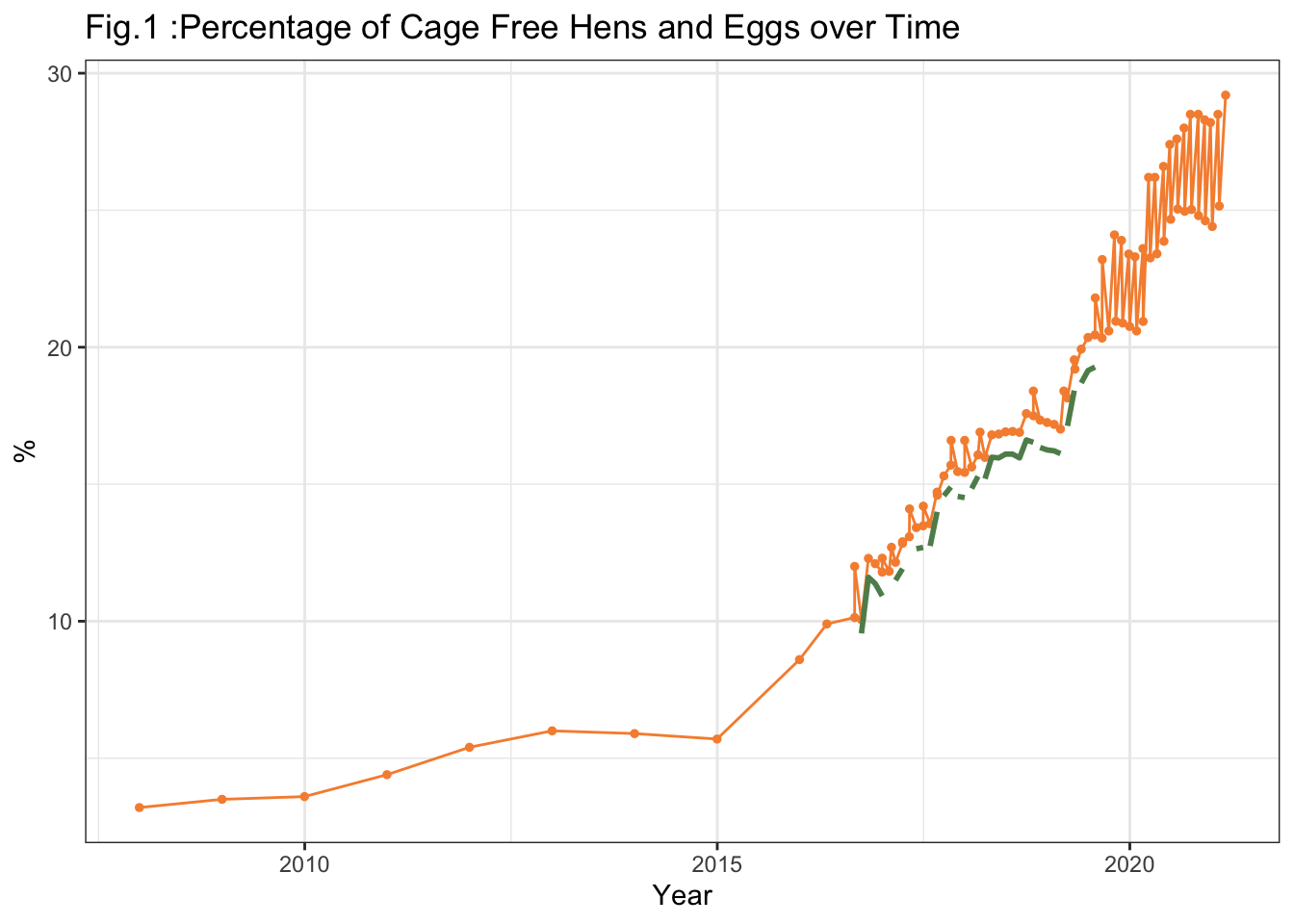
Percentage of Hens are in orange, and percentage of eggs are in green. We see an increase in percentage of cage free eggs and hens over time.

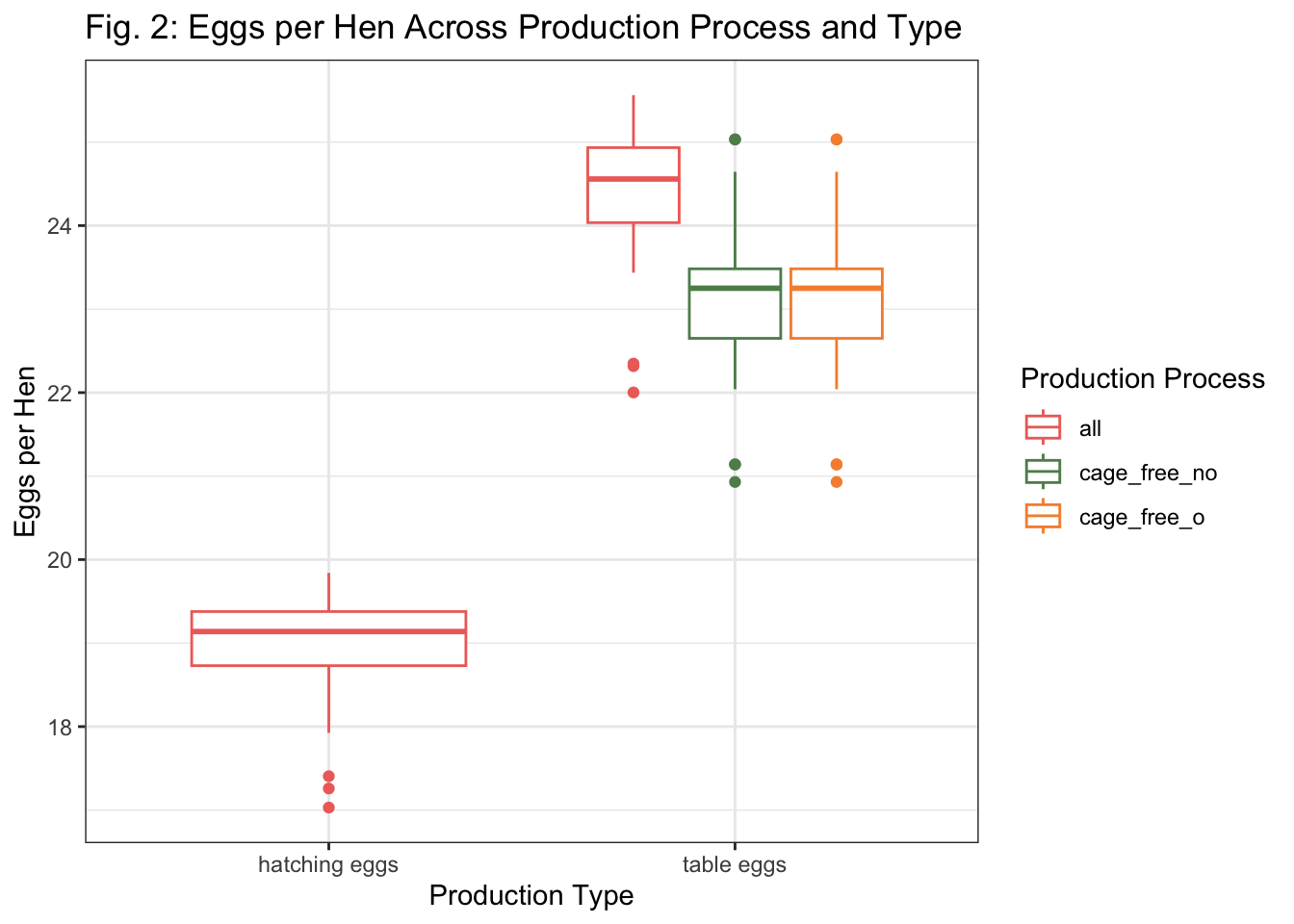
Fig. 2: Eggs per Hen across production type and process

egg %>%
  ggplot() + geom_boxplot(
    aes(x = prod_type,
        y = egg_hen,
        color = prod_process)) +
  theme_bw()+
  labs(title = "Fig. 2: Eggs per Hen Across Production Process and Type",
       x = "Production Type",
       y = "Eggs per Hen",
       color = "Production Process") + 
  scale_color_manual(values = c(all = "#ee6f68",
                                cage_free_no = "#5e8d5a",
                                cage_free_o = "#f68f3c"))

Figure 2 depicts a stark difference in the number eggs per hen between hatching eggs and table eggs. No difference is observed between the production processes within the table eggs.

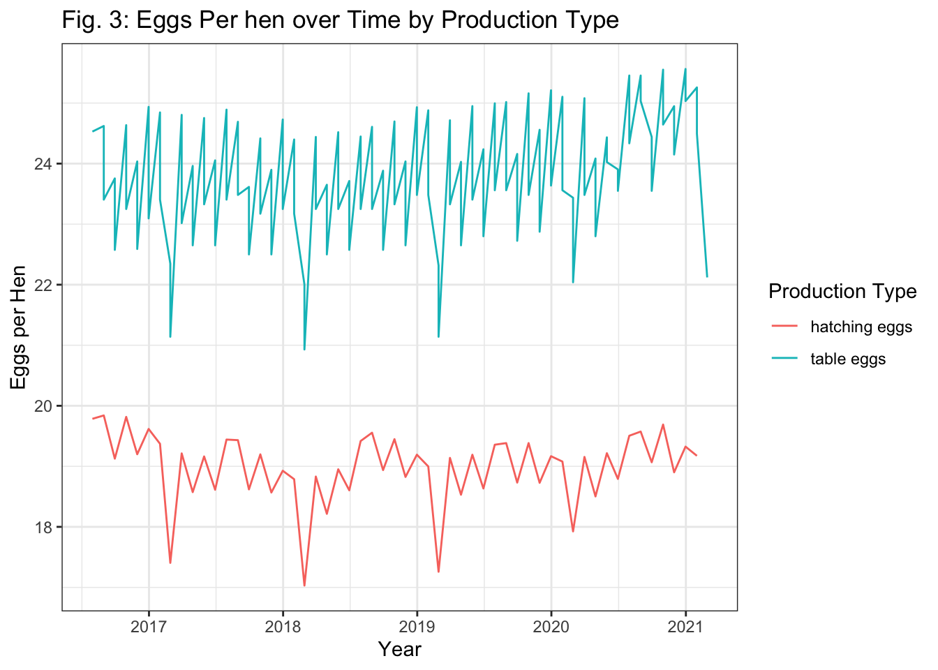
Fig. 3: Eggs per hen over time

egg %>%
  ggplot() + geom_line(
    aes(x = observed_month,
        y = egg_hen,
        color = prod_type)) +
  theme_bw()+
  labs(x = "Year",
       y = "Eggs per Hen",
       title = "Fig. 3: Eggs Per hen over Time by Production Type",
       color = "Production Type")

Similarly, Figure 3 shows that more eggs per hen are produced from the table eggs process.

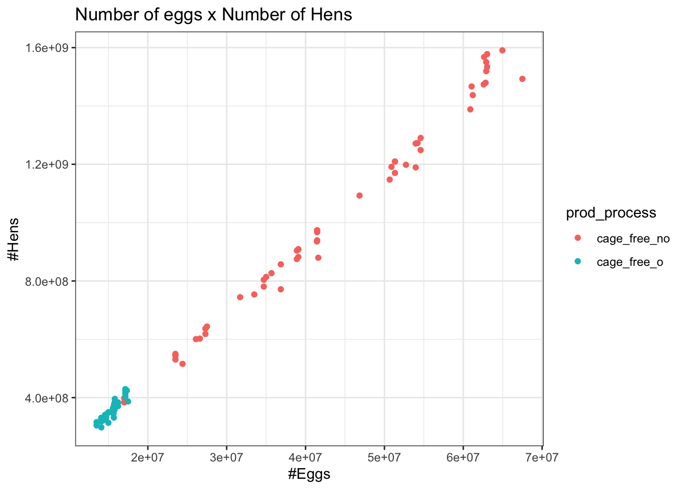
Fig.4 Eggs x Hens

p<- egg %>%
  filter(prod_type %in% "table eggs",
         !prod_process %in% "all") 
p %>%
  ggplot() + geom_point(
    aes(x = n_hens,
        y = n_eggs,
    color = prod_process)) +
  theme_bw()+
  labs(x = "#Eggs",
       y = "#Hens",
       title = "Number of eggs x Number of Hens")

This is a very linear correlation- but not a very interesting question.

Question/Hypothesis:

Because a higher portion of the population consumes eggs as opposed to hatching chicks, and due to the energetically taxing/limiting process of hatching, we expect to see a significantly higher effort towards the production of table eggs as opposed to hatching eggs.

Predictor: Production Type (Hatching or Table Eggs)
Outcome: Eggs per hen

Final Cleaning

We will use only the egg dataset.

Remove Columns that are not needed for analysis

egg <- 
  egg %>%
  select(prod_type, egg_hen)

Split into Test and Train Set

# Fix the random numbers by setting the seed 
# This enables the analysis to be reproducible when random numbers are used 
set.seed(222)
# Put 3/4 of the data into the training set 
data_split <- initial_split(egg, prop = 3/4)

# Create data frames for the two sets:
train <- training(data_split)
test  <- testing(data_split)

Modeling

0. NULL MODEL

5-Fold Cross Validation

fold_egg_train <- vfold_cv(train, v = 5, repeats = 5, strata = egg_hen)

fold_egg_test <- vfold_cv(test, v = 5, repeats = 5, strata = egg_hen)

Warning: The number of observations in each quantile is below the recommended threshold of 20.
• Stratification will use 2 breaks instead.
The number of observations in each quantile is below the recommended threshold of 20.
• Stratification will use 2 breaks instead.
The number of observations in each quantile is below the recommended threshold of 20.
• Stratification will use 2 breaks instead.
The number of observations in each quantile is below the recommended threshold of 20.
• Stratification will use 2 breaks instead.
The number of observations in each quantile is below the recommended threshold of 20.
• Stratification will use 2 breaks instead.

Recipes

#Train Data
egg_rec_train <- 
  recipe(egg_hen ~ prod_type, data = train)# %>%
 # step_dummy(all_nominal(), -all_outcomes()) %>% 
 # step_ordinalscore() %>%
 # step_zv(all_predictors()) 


#Test Data
egg_rec_test <- 
 recipe(egg_hen ~ prod_type, data = test) #%>%
 # step_dummy(all_nominal(), -all_outcomes()) %>%
#  step_ordinalscore() %>%
 # step_zv(all_predictors())

Define Model

lm_mod <- 
  linear_reg() %>% 
  set_engine("lm") %>% 
  set_mode("regression")

Train Data

Recipe

null_train_rec<- 
recipe(egg_hen ~ 1, data = train)

null_train_rec

── Recipe ──────────────────────────────────────────────────────────────────────

── Inputs

Number of variables by role

outcome: 1

Workflow

null_train_wf <- 
  workflow() %>% 
  add_model(lm_mod) %>% 
  add_recipe(null_train_rec)

Fit

null_train_fit <- 
  fit_resamples(null_train_wf, resamples = fold_egg_train)

! Fold1, Repeat1: internal:
  There was 1 warning in `dplyr::summarise()`.
  ℹ In argument: `.estimate = metric_fn(truth = egg_hen, estimate = .pre...
    = na_rm)`.
  Caused by warning:
  ! A correlation computation is required, but `estimate` is constant an...

! Fold2, Repeat1: internal:
  There was 1 warning in `dplyr::summarise()`.
  ℹ In argument: `.estimate = metric_fn(truth = egg_hen, estimate = .pre...
    = na_rm)`.
  Caused by warning:
  ! A correlation computation is required, but `estimate` is constant an...

! Fold3, Repeat1: internal:
  There was 1 warning in `dplyr::summarise()`.
  ℹ In argument: `.estimate = metric_fn(truth = egg_hen, estimate = .pre...
    = na_rm)`.
  Caused by warning:
  ! A correlation computation is required, but `estimate` is constant an...

! Fold4, Repeat1: internal:
  There was 1 warning in `dplyr::summarise()`.
  ℹ In argument: `.estimate = metric_fn(truth = egg_hen, estimate = .pre...
    = na_rm)`.
  Caused by warning:
  ! A correlation computation is required, but `estimate` is constant an...

! Fold5, Repeat1: internal:
  There was 1 warning in `dplyr::summarise()`.
  ℹ In argument: `.estimate = metric_fn(truth = egg_hen, estimate = .pre...
    = na_rm)`.
  Caused by warning:
  ! A correlation computation is required, but `estimate` is constant an...

! Fold1, Repeat2: internal:
  There was 1 warning in `dplyr::summarise()`.
  ℹ In argument: `.estimate = metric_fn(truth = egg_hen, estimate = .pre...
    = na_rm)`.
  Caused by warning:
  ! A correlation computation is required, but `estimate` is constant an...

! Fold2, Repeat2: internal:
  There was 1 warning in `dplyr::summarise()`.
  ℹ In argument: `.estimate = metric_fn(truth = egg_hen, estimate = .pre...
    = na_rm)`.
  Caused by warning:
  ! A correlation computation is required, but `estimate` is constant an...

! Fold3, Repeat2: internal:
  There was 1 warning in `dplyr::summarise()`.
  ℹ In argument: `.estimate = metric_fn(truth = egg_hen, estimate = .pre...
    = na_rm)`.
  Caused by warning:
  ! A correlation computation is required, but `estimate` is constant an...

! Fold4, Repeat2: internal:
  There was 1 warning in `dplyr::summarise()`.
  ℹ In argument: `.estimate = metric_fn(truth = egg_hen, estimate = .pre...
    = na_rm)`.
  Caused by warning:
  ! A correlation computation is required, but `estimate` is constant an...

! Fold5, Repeat2: internal:
  There was 1 warning in `dplyr::summarise()`.
  ℹ In argument: `.estimate = metric_fn(truth = egg_hen, estimate = .pre...
    = na_rm)`.
  Caused by warning:
  ! A correlation computation is required, but `estimate` is constant an...

! Fold1, Repeat3: internal:
  There was 1 warning in `dplyr::summarise()`.
  ℹ In argument: `.estimate = metric_fn(truth = egg_hen, estimate = .pre...
    = na_rm)`.
  Caused by warning:
  ! A correlation computation is required, but `estimate` is constant an...

! Fold2, Repeat3: internal:
  There was 1 warning in `dplyr::summarise()`.
  ℹ In argument: `.estimate = metric_fn(truth = egg_hen, estimate = .pre...
    = na_rm)`.
  Caused by warning:
  ! A correlation computation is required, but `estimate` is constant an...

! Fold3, Repeat3: internal:
  There was 1 warning in `dplyr::summarise()`.
  ℹ In argument: `.estimate = metric_fn(truth = egg_hen, estimate = .pre...
    = na_rm)`.
  Caused by warning:
  ! A correlation computation is required, but `estimate` is constant an...

! Fold4, Repeat3: internal:
  There was 1 warning in `dplyr::summarise()`.
  ℹ In argument: `.estimate = metric_fn(truth = egg_hen, estimate = .pre...
    = na_rm)`.
  Caused by warning:
  ! A correlation computation is required, but `estimate` is constant an...

! Fold5, Repeat3: internal:
  There was 1 warning in `dplyr::summarise()`.
  ℹ In argument: `.estimate = metric_fn(truth = egg_hen, estimate = .pre...
    = na_rm)`.
  Caused by warning:
  ! A correlation computation is required, but `estimate` is constant an...

! Fold1, Repeat4: internal:
  There was 1 warning in `dplyr::summarise()`.
  ℹ In argument: `.estimate = metric_fn(truth = egg_hen, estimate = .pre...
    = na_rm)`.
  Caused by warning:
  ! A correlation computation is required, but `estimate` is constant an...

! Fold2, Repeat4: internal:
  There was 1 warning in `dplyr::summarise()`.
  ℹ In argument: `.estimate = metric_fn(truth = egg_hen, estimate = .pre...
    = na_rm)`.
  Caused by warning:
  ! A correlation computation is required, but `estimate` is constant an...

! Fold3, Repeat4: internal:
  There was 1 warning in `dplyr::summarise()`.
  ℹ In argument: `.estimate = metric_fn(truth = egg_hen, estimate = .pre...
    = na_rm)`.
  Caused by warning:
  ! A correlation computation is required, but `estimate` is constant an...

! Fold4, Repeat4: internal:
  There was 1 warning in `dplyr::summarise()`.
  ℹ In argument: `.estimate = metric_fn(truth = egg_hen, estimate = .pre...
    = na_rm)`.
  Caused by warning:
  ! A correlation computation is required, but `estimate` is constant an...

! Fold5, Repeat4: internal:
  There was 1 warning in `dplyr::summarise()`.
  ℹ In argument: `.estimate = metric_fn(truth = egg_hen, estimate = .pre...
    = na_rm)`.
  Caused by warning:
  ! A correlation computation is required, but `estimate` is constant an...

! Fold1, Repeat5: internal:
  There was 1 warning in `dplyr::summarise()`.
  ℹ In argument: `.estimate = metric_fn(truth = egg_hen, estimate = .pre...
    = na_rm)`.
  Caused by warning:
  ! A correlation computation is required, but `estimate` is constant an...

! Fold2, Repeat5: internal:
  There was 1 warning in `dplyr::summarise()`.
  ℹ In argument: `.estimate = metric_fn(truth = egg_hen, estimate = .pre...
    = na_rm)`.
  Caused by warning:
  ! A correlation computation is required, but `estimate` is constant an...

! Fold3, Repeat5: internal:
  There was 1 warning in `dplyr::summarise()`.
  ℹ In argument: `.estimate = metric_fn(truth = egg_hen, estimate = .pre...
    = na_rm)`.
  Caused by warning:
  ! A correlation computation is required, but `estimate` is constant an...

! Fold4, Repeat5: internal:
  There was 1 warning in `dplyr::summarise()`.
  ℹ In argument: `.estimate = metric_fn(truth = egg_hen, estimate = .pre...
    = na_rm)`.
  Caused by warning:
  ! A correlation computation is required, but `estimate` is constant an...

! Fold5, Repeat5: internal:
  There was 1 warning in `dplyr::summarise()`.
  ℹ In argument: `.estimate = metric_fn(truth = egg_hen, estimate = .pre...
    = na_rm)`.
  Caused by warning:
  ! A correlation computation is required, but `estimate` is constant an...

RMSE Metric

null_train_met <- collect_metrics(null_train_fit)

null_train_met

# A tibble: 2 × 6
  .metric .estimator   mean     n std_err .config             
  <chr>   <chr>       <dbl> <int>   <dbl> <chr>               
1 rmse    standard     2.18    25  0.0106 Preprocessor1_Model1
2 rsq     standard   NaN        0 NA      Preprocessor1_Model1

RMSE = 2.18 and STD_ERR = 0.011

Test Data

Recipe

null_test_rec<- 
  recipe(egg_hen ~ 1, data = test)

Workflow

null_test_wf <- 
  workflow() %>% 
  add_model(lm_mod) %>% 
  add_recipe(null_test_rec)

Fit

null_test_fit <- 
  fit_resamples(null_test_wf, resamples = fold_egg_test)

! Fold1, Repeat1: internal:
  There was 1 warning in `dplyr::summarise()`.
  ℹ In argument: `.estimate = metric_fn(truth = egg_hen, estimate = .pre...
    = na_rm)`.
  Caused by warning:
  ! A correlation computation is required, but `estimate` is constant an...

! Fold2, Repeat1: internal:
  There was 1 warning in `dplyr::summarise()`.
  ℹ In argument: `.estimate = metric_fn(truth = egg_hen, estimate = .pre...
    = na_rm)`.
  Caused by warning:
  ! A correlation computation is required, but `estimate` is constant an...

! Fold3, Repeat1: internal:
  There was 1 warning in `dplyr::summarise()`.
  ℹ In argument: `.estimate = metric_fn(truth = egg_hen, estimate = .pre...
    = na_rm)`.
  Caused by warning:
  ! A correlation computation is required, but `estimate` is constant an...

! Fold4, Repeat1: internal:
  There was 1 warning in `dplyr::summarise()`.
  ℹ In argument: `.estimate = metric_fn(truth = egg_hen, estimate = .pre...
    = na_rm)`.
  Caused by warning:
  ! A correlation computation is required, but `estimate` is constant an...

! Fold5, Repeat1: internal:
  There was 1 warning in `dplyr::summarise()`.
  ℹ In argument: `.estimate = metric_fn(truth = egg_hen, estimate = .pre...
    = na_rm)`.
  Caused by warning:
  ! A correlation computation is required, but `estimate` is constant an...

! Fold1, Repeat2: internal:
  There was 1 warning in `dplyr::summarise()`.
  ℹ In argument: `.estimate = metric_fn(truth = egg_hen, estimate = .pre...
    = na_rm)`.
  Caused by warning:
  ! A correlation computation is required, but `estimate` is constant an...

! Fold2, Repeat2: internal:
  There was 1 warning in `dplyr::summarise()`.
  ℹ In argument: `.estimate = metric_fn(truth = egg_hen, estimate = .pre...
    = na_rm)`.
  Caused by warning:
  ! A correlation computation is required, but `estimate` is constant an...

! Fold3, Repeat2: internal:
  There was 1 warning in `dplyr::summarise()`.
  ℹ In argument: `.estimate = metric_fn(truth = egg_hen, estimate = .pre...
    = na_rm)`.
  Caused by warning:
  ! A correlation computation is required, but `estimate` is constant an...

! Fold4, Repeat2: internal:
  There was 1 warning in `dplyr::summarise()`.
  ℹ In argument: `.estimate = metric_fn(truth = egg_hen, estimate = .pre...
    = na_rm)`.
  Caused by warning:
  ! A correlation computation is required, but `estimate` is constant an...

! Fold5, Repeat2: internal:
  There was 1 warning in `dplyr::summarise()`.
  ℹ In argument: `.estimate = metric_fn(truth = egg_hen, estimate = .pre...
    = na_rm)`.
  Caused by warning:
  ! A correlation computation is required, but `estimate` is constant an...

! Fold1, Repeat3: internal:
  There was 1 warning in `dplyr::summarise()`.
  ℹ In argument: `.estimate = metric_fn(truth = egg_hen, estimate = .pre...
    = na_rm)`.
  Caused by warning:
  ! A correlation computation is required, but `estimate` is constant an...

! Fold2, Repeat3: internal:
  There was 1 warning in `dplyr::summarise()`.
  ℹ In argument: `.estimate = metric_fn(truth = egg_hen, estimate = .pre...
    = na_rm)`.
  Caused by warning:
  ! A correlation computation is required, but `estimate` is constant an...

! Fold3, Repeat3: internal:
  There was 1 warning in `dplyr::summarise()`.
  ℹ In argument: `.estimate = metric_fn(truth = egg_hen, estimate = .pre...
    = na_rm)`.
  Caused by warning:
  ! A correlation computation is required, but `estimate` is constant an...

! Fold4, Repeat3: internal:
  There was 1 warning in `dplyr::summarise()`.
  ℹ In argument: `.estimate = metric_fn(truth = egg_hen, estimate = .pre...
    = na_rm)`.
  Caused by warning:
  ! A correlation computation is required, but `estimate` is constant an...

! Fold5, Repeat3: internal:
  There was 1 warning in `dplyr::summarise()`.
  ℹ In argument: `.estimate = metric_fn(truth = egg_hen, estimate = .pre...
    = na_rm)`.
  Caused by warning:
  ! A correlation computation is required, but `estimate` is constant an...

! Fold1, Repeat4: internal:
  There was 1 warning in `dplyr::summarise()`.
  ℹ In argument: `.estimate = metric_fn(truth = egg_hen, estimate = .pre...
    = na_rm)`.
  Caused by warning:
  ! A correlation computation is required, but `estimate` is constant an...

! Fold2, Repeat4: internal:
  There was 1 warning in `dplyr::summarise()`.
  ℹ In argument: `.estimate = metric_fn(truth = egg_hen, estimate = .pre...
    = na_rm)`.
  Caused by warning:
  ! A correlation computation is required, but `estimate` is constant an...

! Fold3, Repeat4: internal:
  There was 1 warning in `dplyr::summarise()`.
  ℹ In argument: `.estimate = metric_fn(truth = egg_hen, estimate = .pre...
    = na_rm)`.
  Caused by warning:
  ! A correlation computation is required, but `estimate` is constant an...

! Fold4, Repeat4: internal:
  There was 1 warning in `dplyr::summarise()`.
  ℹ In argument: `.estimate = metric_fn(truth = egg_hen, estimate = .pre...
    = na_rm)`.
  Caused by warning:
  ! A correlation computation is required, but `estimate` is constant an...

! Fold5, Repeat4: internal:
  There was 1 warning in `dplyr::summarise()`.
  ℹ In argument: `.estimate = metric_fn(truth = egg_hen, estimate = .pre...
    = na_rm)`.
  Caused by warning:
  ! A correlation computation is required, but `estimate` is constant an...

! Fold1, Repeat5: internal:
  There was 1 warning in `dplyr::summarise()`.
  ℹ In argument: `.estimate = metric_fn(truth = egg_hen, estimate = .pre...
    = na_rm)`.
  Caused by warning:
  ! A correlation computation is required, but `estimate` is constant an...

! Fold2, Repeat5: internal:
  There was 1 warning in `dplyr::summarise()`.
  ℹ In argument: `.estimate = metric_fn(truth = egg_hen, estimate = .pre...
    = na_rm)`.
  Caused by warning:
  ! A correlation computation is required, but `estimate` is constant an...

! Fold3, Repeat5: internal:
  There was 1 warning in `dplyr::summarise()`.
  ℹ In argument: `.estimate = metric_fn(truth = egg_hen, estimate = .pre...
    = na_rm)`.
  Caused by warning:
  ! A correlation computation is required, but `estimate` is constant an...

! Fold4, Repeat5: internal:
  There was 1 warning in `dplyr::summarise()`.
  ℹ In argument: `.estimate = metric_fn(truth = egg_hen, estimate = .pre...
    = na_rm)`.
  Caused by warning:
  ! A correlation computation is required, but `estimate` is constant an...

! Fold5, Repeat5: internal:
  There was 1 warning in `dplyr::summarise()`.
  ℹ In argument: `.estimate = metric_fn(truth = egg_hen, estimate = .pre...
    = na_rm)`.
  Caused by warning:
  ! A correlation computation is required, but `estimate` is constant an...

Metrics: RMSE

null_test_met <- collect_metrics(null_test_fit)

null_test_met

# A tibble: 2 × 6
  .metric .estimator   mean     n std_err .config             
  <chr>   <chr>       <dbl> <int>   <dbl> <chr>               
1 rmse    standard     2.19    25  0.0838 Preprocessor1_Model1
2 rsq     standard   NaN        0 NA      Preprocessor1_Model1

RMSE = 2.19 and STD_ERR = 0.084

1. LINEAR MODEL

Run Model

#Set up linear model
lm_mod<- linear_reg() %>%
  set_engine("lm") %>%
  set_mode("regression")

#Workflow that adds recipe to model
lm_wflow<- 
  workflow() %>%
  add_model(lm_mod) %>%
  add_recipe(egg_rec_train)

#Use workflow to fit model to  data set
egg_fit<- lm_wflow %>%
  fit(data = train)

#View as Tibble 
egg_fit %>%
  extract_fit_parsnip() %>%
  tidy()

# A tibble: 2 × 5
  term                estimate std.error statistic   p.value
  <chr>                  <dbl>     <dbl>     <dbl>     <dbl>
1 (Intercept)            19.0      0.134     142.  9.30e-173
2 prod_typetable eggs     4.55     0.156      29.2 1.15e- 66

Assess Performance

RMSE

aug_test <- augment(egg_fit, train)
rmse <- aug_test %>% rmse(truth = egg_hen, .pred)
rsq <- aug_test %>% rsq(truth = egg_hen, .pred)
metrics<- full_join(rmse, rsq)

Joining with `by = join_by(.metric, .estimator, .estimate)`

metrics

# A tibble: 2 × 3
  .metric .estimator .estimate
  <chr>   <chr>          <dbl>
1 rmse    standard       0.873
2 rsq     standard       0.840

RMSE = 0.87

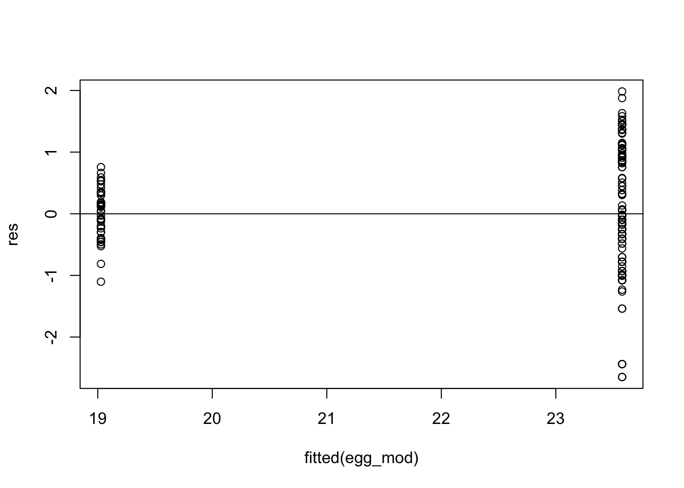
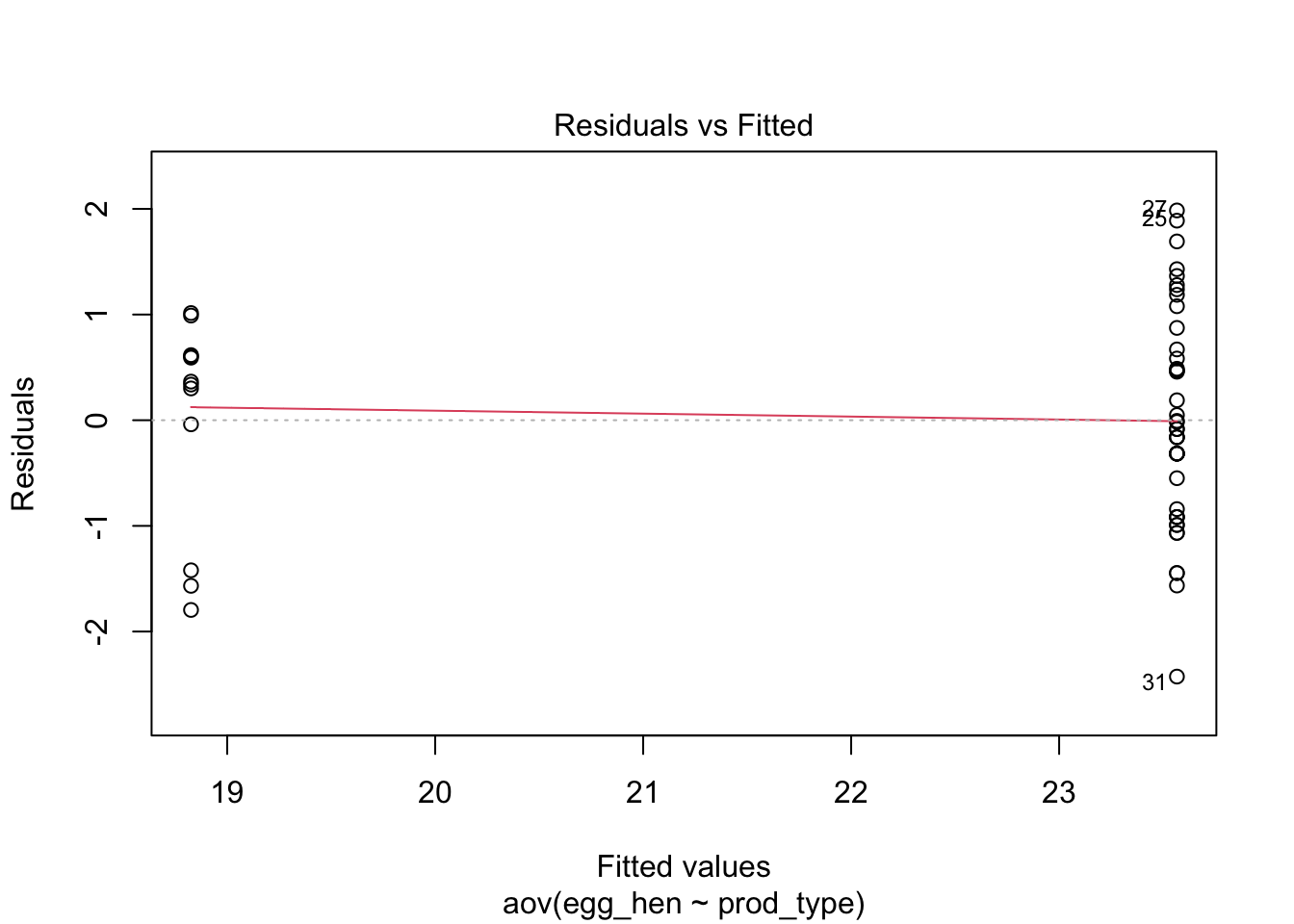
Residuals

egg_mod<- lm(egg_hen ~ prod_type, data = train)
res<- resid(egg_mod)
plot(fitted(egg_mod), res)
abline(0,0)

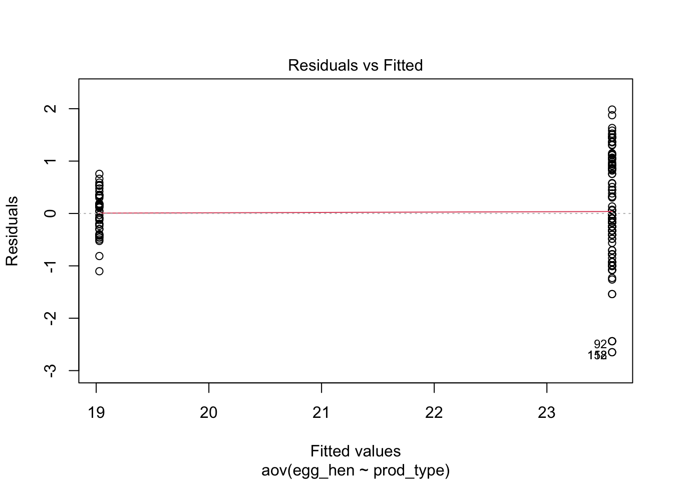
2. ANOVA MODEL

ANOVA is a statistical test for estimating how a quantitative dependent variable changes according to the levels of one or more categorical independent variables. ANOVA tests whether there is a difference in means of the groups at each level of the independent variable.

Null

#Model
anova_n<- 
  aov(egg_hen ~ 1, data = egg)
summary(anova_n)

             Df Sum Sq Mean Sq F value Pr(>F)
Residuals   219   1050   4.796

#Assess Performance
RSS<- c(crossprod(anova_n$residuals))
MSE<- RSS / length(anova_n$residuals)
RMSE <- sqrt(MSE)
RMSE

[1] 2.185032

RMSE of Null = 2.18

Actual Model

#Model
anova<- 
  aov(egg_hen ~ prod_type, data = train)
summary(anova)

             Df Sum Sq Mean Sq F value Pr(>F)    
prod_type     1  658.4   658.4   853.1 <2e-16 ***
Residuals   163  125.8     0.8                   
---
Signif. codes:  0 '***' 0.001 '**' 0.01 '*' 0.05 '.' 0.1 ' ' 1

#Assess Performance
RSS<- c(crossprod(anova$residuals))
MSE<- RSS / length(anova$residuals)
RMSE <- sqrt(MSE)
RMSE

[1] 0.873181

RMSE for Actual Model = 0.87

Plot

plot(anova, 1)

3. TREE MODEL

Model Specification

tune_spec_dtree <- 
  decision_tree(
    cost_complexity = tune(),
    tree_depth = tune()) %>%
  set_engine("rpart") %>% 
  set_mode("regression")

tune_spec_dtree

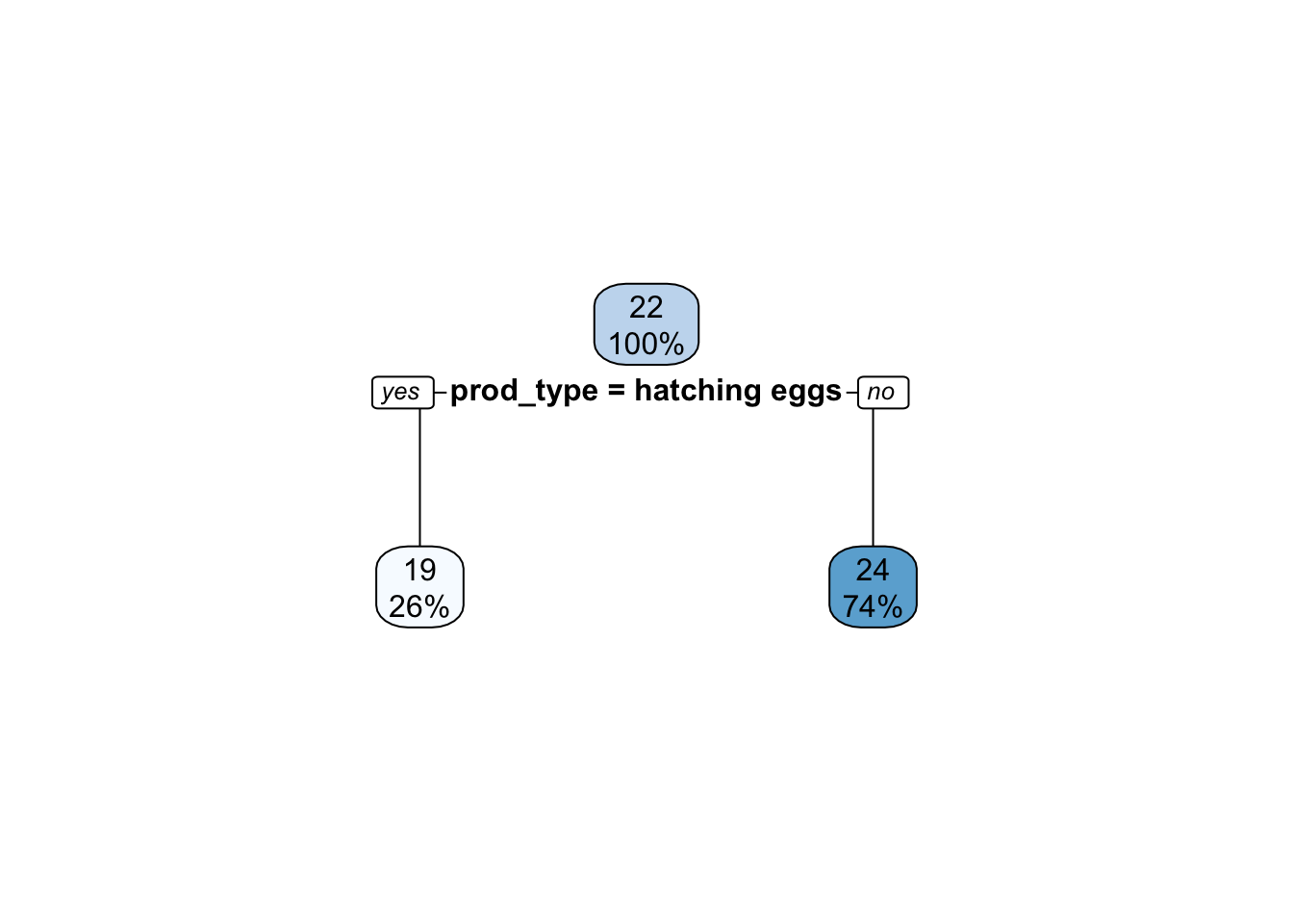
Decision Tree Model Specification (regression)

Main Arguments:
  cost_complexity = tune()
  tree_depth = tune()

Computational engine: rpart

Think of tune() here as a placeholder. After the tuning process, we will select a single numeric value for each of these hyperparameters. For now, we specify our parsnip model object and identify the hyperparameters we will tune().

Workflow Definition

dtree_wf <- workflow() %>%
  add_model(tune_spec_dtree) %>%
  add_recipe(egg_rec_train)

Tuning Grid Specification

We can create a regular grid of values to try using some convenience functions for each hyperparameter:

#create a regular grid of values for using convenience functions for each hyperparameter.
tree_grid_dtree <-
  grid_regular(
    cost_complexity(), 
    tree_depth(), 
    levels = 5)

tree_grid_dtree

# A tibble: 25 × 2
   cost_complexity tree_depth
             <dbl>      <int>
 1    0.0000000001          1
 2    0.0000000178          1
 3    0.00000316            1
 4    0.000562              1
 5    0.1                   1
 6    0.0000000001          4
 7    0.0000000178          4
 8    0.00000316            4
 9    0.000562              4
10    0.1                   4
# … with 15 more rows

Tuning using Cross-validation and `tune_grid()` function

dtree_resample <- 
  dtree_wf %>% 
  tune_grid(
    resamples = fold_egg_train,
    grid = tree_grid_dtree)

Once we have our tuning results, we can both explore them through visualization and then select the best result. The function collect_metrics() gives us a tidy tibble with all the results

dtree_resample %>%
  collect_metrics()

# A tibble: 50 × 8
   cost_complexity tree_depth .metric .estimator  mean     n std_err .config    
             <dbl>      <int> <chr>   <chr>      <dbl> <int>   <dbl> <chr>      
 1    0.0000000001          1 rmse    standard   0.872    25 0.0152  Preprocess…
 2    0.0000000001          1 rsq     standard   0.841    25 0.00563 Preprocess…
 3    0.0000000178          1 rmse    standard   0.872    25 0.0152  Preprocess…
 4    0.0000000178          1 rsq     standard   0.841    25 0.00563 Preprocess…
 5    0.00000316            1 rmse    standard   0.872    25 0.0152  Preprocess…
 6    0.00000316            1 rsq     standard   0.841    25 0.00563 Preprocess…
 7    0.000562              1 rmse    standard   0.872    25 0.0152  Preprocess…
 8    0.000562              1 rsq     standard   0.841    25 0.00563 Preprocess…
 9    0.1                   1 rmse    standard   0.872    25 0.0152  Preprocess…
10    0.1                   1 rsq     standard   0.841    25 0.00563 Preprocess…
# … with 40 more rows

Plot Model using autoplot()

dtree_resample %>%
  collect_metrics() %>%
  mutate(tree_depth = factor(tree_depth)) %>%
  ggplot(aes(cost_complexity, mean, color = tree_depth)) +
  geom_line(linewidth = 1.5, alpha = 0.6) +
  geom_point(size = 2) +
  facet_wrap(~ .metric, scales = "free", nrow = 2) +
  scale_x_log10(labels = scales::label_number()) +
  scale_color_viridis_d(option = "plasma", begin = .9, end = 0)

Metrics: RMSE

The show_best() function shows us the top 5 candidate models by default. We set n=1

dtree_resample %>%
  show_best(n=1)

Warning: No value of `metric` was given; metric 'rmse' will be used.

# A tibble: 1 × 8
  cost_complexity tree_depth .metric .estimator  mean     n std_err .config     
            <dbl>      <int> <chr>   <chr>      <dbl> <int>   <dbl> <chr>       
1    0.0000000001          1 rmse    standard   0.872    25  0.0152 Preprocesso…

RMSE 0.87 STD_ERR = 0.015

We can also use the select_best() function to pull out the single set of hyperparameter values for our best decision tree model:

#Selects best performing model
best_tree <- dtree_resample %>%
  select_best()

Warning: No value of `metric` was given; metric 'rmse' will be used.

best_tree

# A tibble: 1 × 3
  cost_complexity tree_depth .config              
            <dbl>      <int> <chr>                
1    0.0000000001          1 Preprocessor1_Model01

Create final fit based on best model permutation and plotting predicted values from that final fit model

We can update (or “finalize”) our workflow object tree_wf with the values from select_best().

dtree_final_wf <- 
  dtree_wf %>% 
  finalize_workflow(best_tree)

dtree_final_wf

══ Workflow ════════════════════════════════════════════════════════════════════
Preprocessor: Recipe
Model: decision_tree()

── Preprocessor ────────────────────────────────────────────────────────────────
0 Recipe Steps

── Model ───────────────────────────────────────────────────────────────────────
Decision Tree Model Specification (regression)

Main Arguments:
  cost_complexity = 1e-10
  tree_depth = 1

Computational engine: rpart

#Create workflow for fitting model to train predictions
dtree_final_fit <- 
  dtree_final_wf %>%
  fit(train)

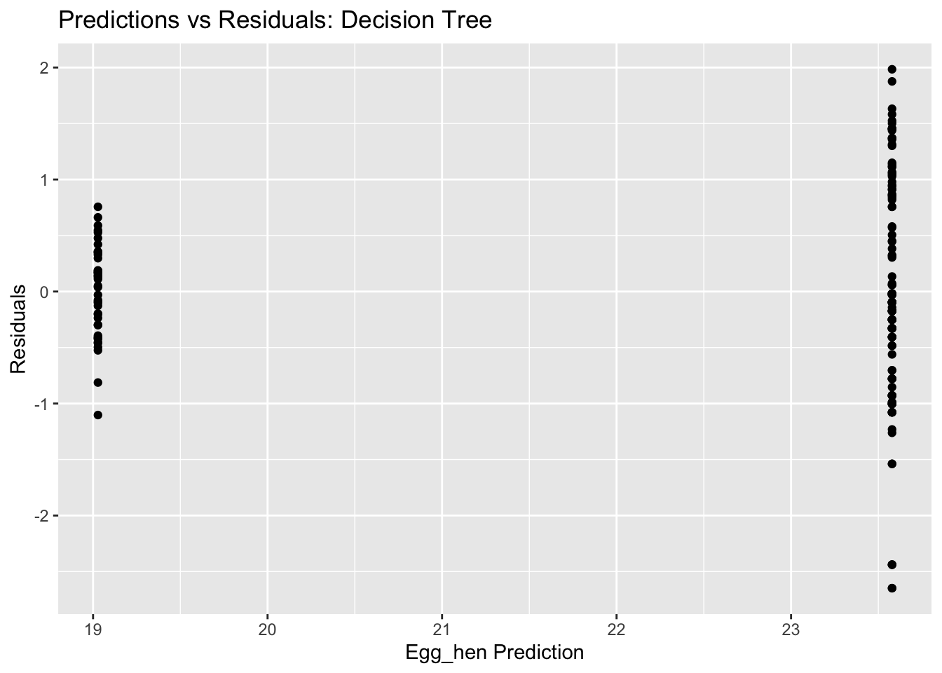
Calculating Residuals and Plotting Actual Vs. Predicted Values

dtree_residuals <- dtree_final_fit %>%
  augment(train) %>% #use augment() to make predictions from train data
  select(c(.pred, egg_hen)) %>%
  mutate(.resid = egg_hen - .pred) #calculate residuals and make new row.

dtree_residuals

# A tibble: 165 × 3
   .pred egg_hen  .resid
   <dbl>   <dbl>   <dbl>
 1  23.6    23.2 -0.406 
 2  23.6    23.6 -0.0187
 3  19.0    18.9 -0.101 
 4  23.6    23.6  0.0588
 5  19.0    18.6 -0.424 
 6  19.0    18.2 -0.813 
 7  23.6    23.4 -0.174 
 8  23.6    23.2 -0.406 
 9  19.0    19.2  0.185 
10  19.0    18.6 -0.454 
# … with 155 more rows

Predictions vs. Actual

dtree_pred_plot <- ggplot(dtree_residuals, 
                          aes(x = egg_hen, 
                              y = .pred)) + 
  geom_point() + 
  labs(title = "Predictions vs Actual: Decision Tree", 
       x = "Egg_hen Outcome", 
       y = "Egg_hen Prediction")
dtree_pred_plot

Predictions vs. Residuals

dtree_residual_plot <- ggplot(dtree_residuals, 
                              aes(y = .resid, 
                                  x = .pred)) + 
  geom_point() + 
  labs(title = "Predictions vs Residuals: Decision Tree", 
       x = "Egg_hen Prediction", 
       y = "Residuals")
plot(dtree_residual_plot) #view plot

4. Regression Decision Tree

Regression Tree

tree <- rpart(egg_hen ~prod_type, data = train)
rpart.plot(tree)

Predict

p <- predict(tree, train)

RMSE and R2

rmse<- sqrt(mean(train$egg_hen - p))
r2<- (cor(train$egg_hen,p))
r2

[1] 0.9162877

rmse

[1] 6.871667e-08

5. Random Forest Model

Create function to detect cores for RFM computation

cores <- parallel::detectCores()
cores

[1] 8

Specify Model

rf_mod <- 
  rand_forest(mtry = tune(), min_n = tune(), trees = 1000) %>% 
  set_engine("ranger", num.threads = cores) %>% 
  set_mode("regression")

Creating Workflow

rf_wf <- workflow() %>%
  add_model(rf_mod) %>%
  add_recipe(egg_rec_train)

Create Tuning Grid

rf_grid  <- expand.grid(mtry = c(3, 4, 5, 6),
                        min_n = c(40,50,60), 
                        trees = c(500,1000)  )

Cross-validation

rf_resample <- 
  rf_wf %>% 
  tune_grid(fold_egg_train,
            grid = 25,
            control = control_grid(save_pred = TRUE),
            metrics = metric_set(yardstick::rmse))

i Creating pre-processing data to finalize unknown parameter: mtry

rf_resample %>%
  collect_metrics()

# A tibble: 23 × 8
    mtry min_n .metric .estimator  mean     n std_err .config              
   <int> <int> <chr>   <chr>      <dbl> <int>   <dbl> <chr>                
 1     1     3 rmse    standard   0.872    25  0.0152 Preprocessor1_Model01
 2     1     9 rmse    standard   0.872    25  0.0153 Preprocessor1_Model02
 3     1    27 rmse    standard   0.872    25  0.0152 Preprocessor1_Model03
 4     1     4 rmse    standard   0.872    25  0.0153 Preprocessor1_Model04
 5     1    13 rmse    standard   0.872    25  0.0152 Preprocessor1_Model05
 6     1    23 rmse    standard   0.872    25  0.0152 Preprocessor1_Model06
 7     1    21 rmse    standard   0.872    25  0.0152 Preprocessor1_Model07
 8     1    35 rmse    standard   0.872    25  0.0153 Preprocessor1_Model08
 9     1    12 rmse    standard   0.872    25  0.0152 Preprocessor1_Model09
10     1     6 rmse    standard   0.872    25  0.0152 Preprocessor1_Model10
# … with 13 more rows

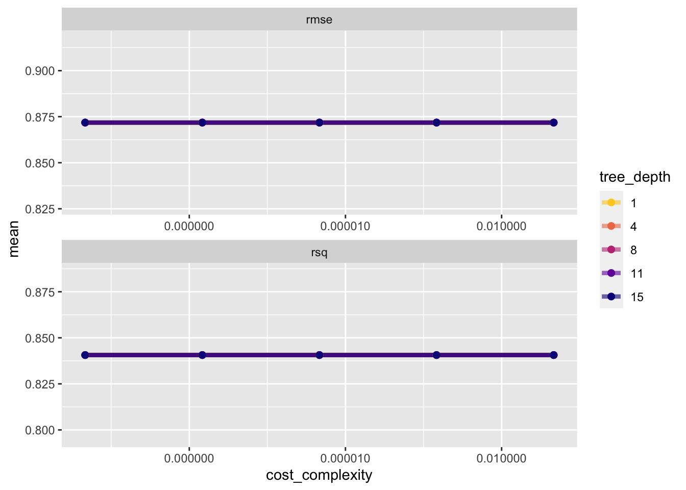
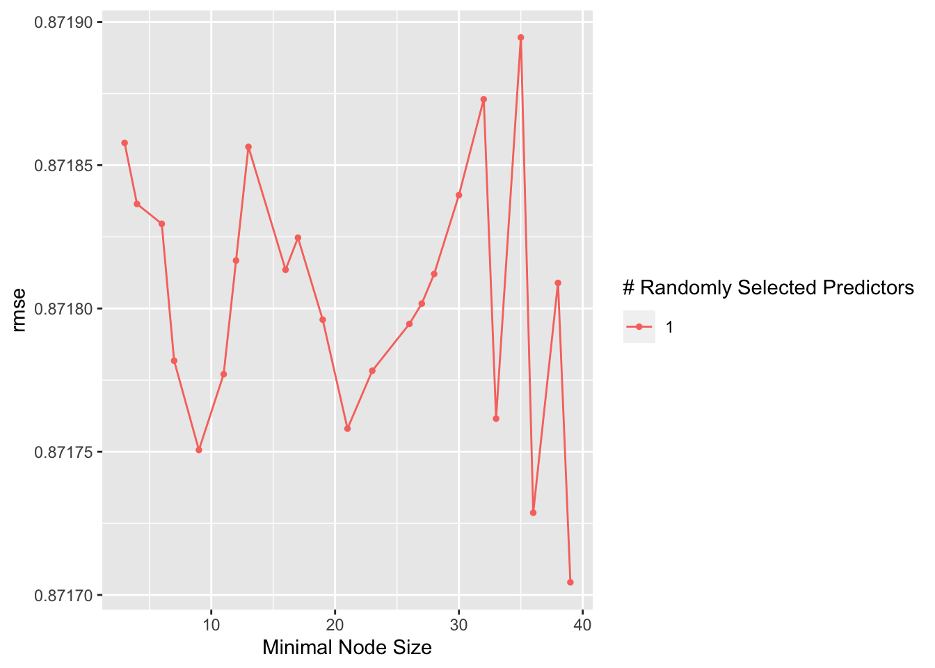
Plot Model Performance

#Plot of actual train data
rf_resample %>%
  autoplot()

Metrics: RMSE

#Showing best performing tree models
rf_resample %>%
  show_best(n=1)

# A tibble: 1 × 8
   mtry min_n .metric .estimator  mean     n std_err .config              
  <int> <int> <chr>   <chr>      <dbl> <int>   <dbl> <chr>                
1     1    39 rmse    standard   0.872    25  0.0152 Preprocessor1_Model22

#Selects best performing model
best_rf <- rf_resample %>%
  select_best(method = "rmse")

RMSE = 0.87 STD_ERR = 0.015

Create Final Fit

rf_final_wf <- 
  rf_wf %>% 
  finalize_workflow(best_rf)

#Create workflow for fitting model to train_data2 predictions
rf_final_fit <- 
  rf_final_wf %>%
  fit(train)

Calculate Residuals

rf_residuals <- rf_final_fit %>%
  augment(train) %>% #use augment() to make predictions from train data
  select(c(.pred, egg_hen)) %>%
  mutate(.resid = egg_hen - .pred) #calculate residuals and make new row.

rf_residuals

# A tibble: 165 × 3
   .pred egg_hen  .resid
   <dbl>   <dbl>   <dbl>
 1  23.6    23.2 -0.408 
 2  23.6    23.6 -0.0202
 3  19.0    18.9 -0.101 
 4  23.6    23.6  0.0574
 5  19.0    18.6 -0.424 
 6  19.0    18.2 -0.813 
 7  23.6    23.4 -0.175 
 8  23.6    23.2 -0.408 
 9  19.0    19.2  0.185 
10  19.0    18.6 -0.454 
# … with 155 more rows

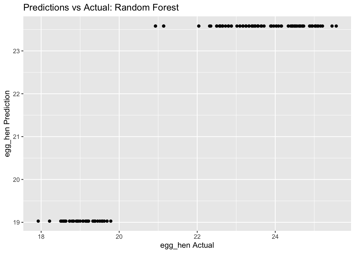
Model Predictions from Tuned Model vs Actual Outcomes

rf_pred_plot <- ggplot(rf_residuals, 
                          aes(x = egg_hen, 
                              y = .pred)) + 
  geom_point() + 
  labs(title = "Predictions vs Actual: Random Forest", 
       x = "egg_hen Actual", 
       y = "egg_hen Prediction")
rf_pred_plot

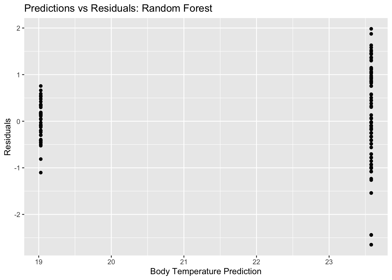
rf_residual_plot <- ggplot(rf_residuals, 
                              aes(y = .resid, 
                                  x = .pred)) + 
  geom_point() + 
  labs(title = "Predictions vs Residuals: Random Forest", 
       x = "Body Temperature Prediction", 
       y = "Residuals")
plot(rf_residual_plot) #view plot

Final Assessment

In order to pick a model that I believe is best for my hypothesis, I must (1) understand the data and question (2) use visual plots, and (3) metrics (e.g. RMSE) to assess performance. Based on these three attributes, I believe that the one-way ANOVA is the best model to use in this case. I am working with a continuous outcome (eggs per hen) and a categorical independent variable (production type) and would like to assess the two means between hatching and table eggs. This model is simple and efficient, and properly addresses the questions. Additionally, the RMSE of the actual model (0.87) was lower than the null model (2.18) indicating a better performance.

The Random Forest Model also had a lower RMSE value (0.87), ut the plot produced depicts a fluctuation in performance with node size. The decision tree is a simple model, but in this case not very informative as we only had two outcomes.

ANOVA on Test Data

#Model
anova_test<- 
  aov(egg_hen ~ prod_type, data = test)
summary(anova_test)

            Df Sum Sq Mean Sq F value Pr(>F)    
prod_type    1 210.81  210.81   204.9 <2e-16 ***
Residuals   53  54.52    1.03                   
---
Signif. codes:  0 '***' 0.001 '**' 0.01 '*' 0.05 '.' 0.1 ' ' 1

#Assess Performance
RSS<- c(crossprod(anova_test$residuals))
MSE<- RSS / length(anova_test$residuals)
RMSE <- sqrt(MSE)
RMSE

[1] 0.9956049

RMSE = 0.99

Plot

plot(anova_test, 1)

Discussion

Data

The data used for this exercise was sourced from The Humane League’s US Egg Production dataset by Samara Mendez. It tracks cage-free hens and the supply of cage-free eggs relative to the overall numbers of hens and table eggs in the United States.

Cleaning

Data cleaning involved making a new column in the egg data set “egg_hen” which represents the number of eggs per hen. Variables within columns were also renamed for convenience.

Visualization

To explore the data, plots were made to depict various trends between the variables (e.g. percentage of cage free hens and eggs over time, eggs per hen over time, eggs per hen across production type/process). From this exploration, we could see a drastic difference in eggs per hen between table and hatching production type. This lead us to explore the relationship between production type (hatching or table) on eggs produced per hen.

Modeling

Final cleaning was conducted (eliminating undesired columns) and the data was split into training and test data (70:30). A null linear model was run for comparison of metrics. Four models were tested in this exercise:

Linear Model
ANOVA Model
Tree Model
Regression Decision Tree
Random Forest Model.

Metrics were run (Primarily RMSE) and compared to the Null model to assess performance. Additionally, visualization methods were used in conjunction with the performance metrics.

Conclusion

Based on the metrics, the question, and the plots, the ANOVA model was chosen, and again run but on the test data. Ultimately, it had a higher RMSE than the train data, but still lower than the null ANOVA, suggesting that this model can be adequate in its ability to address our question.

Getting Started

Libraries

Load Data

Look at Data sets

Initial Cleaning

Cage Data set

Egg Data set

Exploratory Visualization

Fig. 1: Percentage of cage free gens and eggs

Fig. 2: Eggs per Hen across production type and process

Fig. 3: Eggs per hen over time

Fig.4 Eggs x Hens

Question/Hypothesis:

Final Cleaning

Remove Columns that are not needed for analysis

Split into Test and Train Set

Modeling

0. NULL MODEL

5-Fold Cross Validation

Recipes

Define Model

Train Data

Recipe

Workflow

Fit

RMSE Metric

Test Data

Recipe

Workflow

Fit

Metrics: RMSE

1. LINEAR MODEL

Run Model

Assess Performance

RMSE

Residuals

2. ANOVA MODEL

Null

Actual Model

Plot

3. TREE MODEL

Model Specification

Workflow Definition

Tuning Grid Specification

Tuning using Cross-validation and tune_grid() function

Plot Model using autoplot()

Metrics: RMSE

Create final fit based on best model permutation and plotting predicted values from that final fit model

Calculating Residuals and Plotting Actual Vs. Predicted Values

Predictions vs. Actual

Predictions vs. Residuals

4. Regression Decision Tree

Regression Tree

Predict

RMSE and R2

5. Random Forest Model

Create function to detect cores for RFM computation

Specify Model

Creating Workflow

Create Tuning Grid

Cross-validation

Plot Model Performance

Metrics: RMSE

Create Final Fit

Calculate Residuals

Model Predictions from Tuned Model vs Actual Outcomes

Final Assessment

ANOVA on Test Data

Plot

Discussion

Data

Cleaning

Visualization

Modeling

Conclusion

Tuning using Cross-validation and `tune_grid()` function