library(tidyverse)
library(here)
library(tidytuesdayR)
library(lubridate)
library(skimr)Tidy Tuesday Exercise
Loading Packages
The Data
tuesdata <- tidytuesdayR::tt_load(2023, week = 7)
Downloading file 1 of 1: `age_gaps.csv`age_gaps <- tuesdata$age_gapsTake a look at the data
glimpse(age_gaps)Rows: 1,155
Columns: 13
$ movie_name <chr> "Harold and Maude", "Venus", "The Quiet American", …
$ release_year <dbl> 1971, 2006, 2002, 1998, 2010, 1992, 2009, 1999, 199…
$ director <chr> "Hal Ashby", "Roger Michell", "Phillip Noyce", "Joe…
$ age_difference <dbl> 52, 50, 49, 45, 43, 42, 40, 39, 38, 38, 36, 36, 35,…
$ couple_number <dbl> 1, 1, 1, 1, 1, 1, 1, 1, 1, 1, 1, 1, 1, 1, 1, 1, 1, …
$ actor_1_name <chr> "Ruth Gordon", "Peter O'Toole", "Michael Caine", "D…
$ actor_2_name <chr> "Bud Cort", "Jodie Whittaker", "Do Thi Hai Yen", "T…
$ character_1_gender <chr> "woman", "man", "man", "man", "man", "man", "man", …
$ character_2_gender <chr> "man", "woman", "woman", "woman", "man", "woman", "…
$ actor_1_birthdate <date> 1896-10-30, 1932-08-02, 1933-03-14, 1930-09-17, 19…
$ actor_2_birthdate <date> 1948-03-29, 1982-06-03, 1982-10-01, 1975-11-08, 19…
$ actor_1_age <dbl> 75, 74, 69, 68, 81, 59, 62, 69, 57, 77, 59, 56, 65,…
$ actor_2_age <dbl> 23, 24, 20, 23, 38, 17, 22, 30, 19, 39, 23, 20, 30,…summary(age_gaps) movie_name release_year director age_difference
Length:1155 Min. :1935 Length:1155 Min. : 0.00
Class :character 1st Qu.:1997 Class :character 1st Qu.: 4.00
Mode :character Median :2004 Mode :character Median : 8.00
Mean :2001 Mean :10.42
3rd Qu.:2012 3rd Qu.:15.00
Max. :2022 Max. :52.00
couple_number actor_1_name actor_2_name character_1_gender
Min. :1.000 Length:1155 Length:1155 Length:1155
1st Qu.:1.000 Class :character Class :character Class :character
Median :1.000 Mode :character Mode :character Mode :character
Mean :1.398
3rd Qu.:2.000
Max. :7.000
character_2_gender actor_1_birthdate actor_2_birthdate actor_1_age
Length:1155 Min. :1889-04-16 Min. :1906-10-06 Min. :18.00
Class :character 1st Qu.:1953-05-16 1st Qu.:1965-03-25 1st Qu.:33.00
Mode :character Median :1964-10-03 Median :1974-07-30 Median :39.00
Mean :1960-09-07 Mean :1971-01-29 Mean :40.64
3rd Qu.:1973-08-07 3rd Qu.:1982-04-07 3rd Qu.:47.00
Max. :1996-06-01 Max. :1996-11-11 Max. :81.00
actor_2_age
Min. :17.00
1st Qu.:25.00
Median :29.00
Mean :30.21
3rd Qu.:34.00
Max. :68.00 It looks like we have data from 1935-2022 that contains the movie, release date, director, each actors age and gender, and their birth-dates. For each couple, the age gap is defined in the age_difference column. Gender of character_1 is the older gender, while gender for character_2 is the younger gender in the relationship.
This dataset seems to be fairly clean, with consistent entries for each variable. So lets think about some analyses we can explore.
Analysis Ideas
1. How has the age gap changed over the years?
2. What is the most common age difference?
3. Are age gaps where the male is older than the female more common? Or vice verse?
4. Do we see a greater age gap between same-gender or opposite-gender couples?
5. When do we start seeing the prevalence of same-gender relationships?
1. How has age gap changed over the years?
Slim down Data
d1 <- age_gaps %>%
  select(release_year, age_difference)
Lets just look at the release year and age gap.
Average gap by year
year_avg<- d1 %>%
group_by(release_year) %>%
summarize_if(is.numeric, mean) %>%
ungroup()
Because multiple movies came out in the same year, we are taking an average of the age gap per year.
Plotting average age gap over the years
year_avg %>%
  ggplot() +
  geom_line(
    aes(
      x = release_year,
      y = age_difference),
    color = "darkgreen")+
  geom_point(
    aes(
      x = release_year,
      y = age_difference),
    color = "darkgreen")+
  theme_bw()+
  labs(
    x = "Release Year",
    y = "Age Gap (years)",
    title = "Age gaps in movies from 1935-2022") +
  theme(
    plot.title = element_text(hjust = 0.5))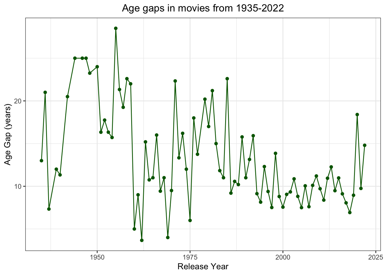
Nothing really stands out here. We see a slight decrease in average age gap between ~1980-2018. the years 2020 and 2022 both had movies with age gaps >20 years (You Should Have Left, Mank, The Northman, and The Bubble).
2. What is the most common age difference?
Let’s make a dataframe that contains the number of times an age gap is reported:
dist<- age_gaps %>%
  count(age_difference)
summary(dist)
age_difference n
Min. : 0.00 Min. : 1.00
1st Qu.:11.25 1st Qu.: 2.25
Median :22.50 Median :16.50
Mean :23.13 Mean :25.11
3rd Qu.:33.75 3rd Qu.:36.75
Max. :52.00 Max. :85.00 Now let’s plot it:
dist %>%
  ggplot() +
  geom_point(
    aes(
      x = age_difference,
      y = n),
    color = "darkblue")+
  geom_line(
    aes(
      x = age_difference,
      y = n),
    color = "darkblue")+
  theme_bw()+
 scale_x_continuous(n.breaks=10)+
  labs(
    x = "Age Gap (years)",
    y = "Number of Times Age Gap Appears",
    title = "Frequency of Age Gaps in Media from 1935-2022" )+
  theme(plot.title = element_text(hjust = 0.5))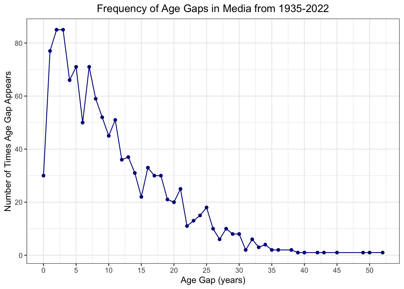
It looks like an age gap of 2-3 years is most common. We also have an age gap of 52 years!
3. Are age gaps where the male is older than the female more common? Or vice verse?
Make new column that identifies the older male or female (character_1_gender refers to gender of older actor)
age_gaps2<- age_gaps %>%
  mutate(older = case_when(age_gaps$character_1_gender == "woman"~ "Female", # Older Female
                           age_gaps$character_1_gender == "man" ~ "Male"))  # Older Male
Plot Age difference over time by gender
age_gaps2 %>% ggplot() + geom_point(
  aes(
    x = release_year,
    y = age_difference,
    color = older))+
  theme_bw()+
  labs(
    x = "Movie Release Year",
    y = "Age Difference",
    title = "Age Difference over Release Years by Gender",
    color = "Older Actor")+
    theme(
      plot.title = element_text(hjust = 0.5))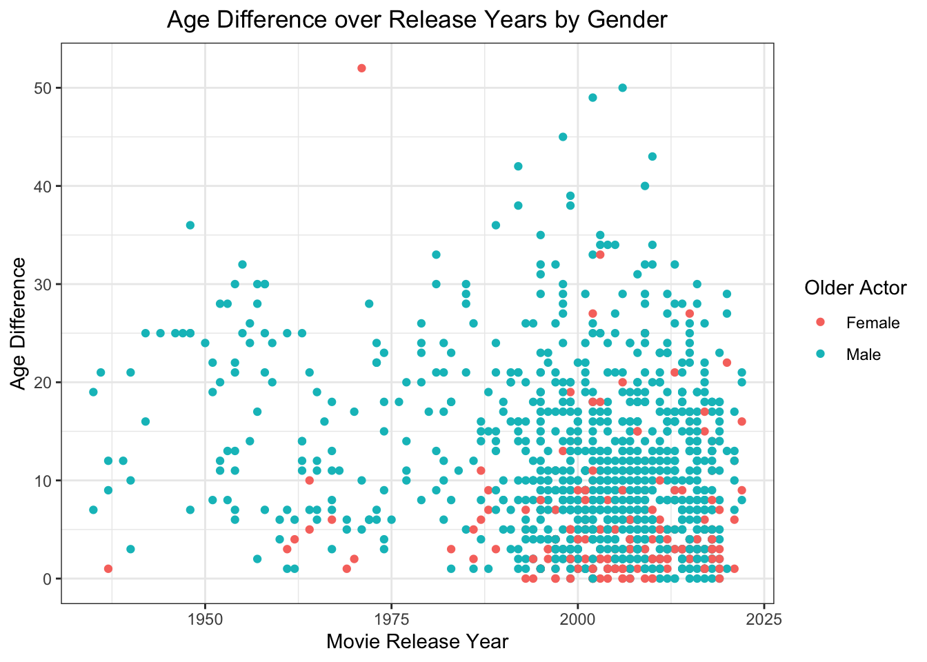
A few things to note here. (1) It looks like older females in couples become more prevalent around the 1980s. (2) Despite a higher incidence of older females in couples, the age gap is relatively lower than that of older male couples. (3) Some of the movies include same-gender couples, which can make this graph misleading. In the case where the couple is woman-woman, older female will show up regardless. So:
Let’s make new columns and dataframes for same and opposite gender couples
age_gaps3<- age_gaps2 %>%
  mutate(gender = case_when(
    #Same-gender male couples
    (age_gaps$character_1_gender == "man" & age_gaps$character_2_gender == "man") ~"same",
    #Same-gender female couples
    (age_gaps$character_1_gender == "woman" & age_gaps$character_2_gender == "woman") ~"same",
    #Opposite-gender couples
    (age_gaps$character_1_gender == "woman" & age_gaps$character_2_gender == "man") ~"opposite",
     #Opposite-gender couples
    (age_gaps$character_1_gender == "man" & age_gaps$character_2_gender == "woman") ~"opposite"))

#New dataframes for same and opposite gender relationships
age_same<- age_gaps3 %>%
  filter(gender %in% "same")

age_opp<- age_gaps3 %>%
filter(gender %in% "opposite")glimpse(age_same)Rows: 23
Columns: 15
$ movie_name <chr> "Beginners", "A Single Man", "Freeheld", "Behind th…
$ release_year <dbl> 2010, 2009, 2015, 2013, 2009, 2009, 2008, 2012, 201…
$ director <chr> "Mike Mills", "Tom Ford", "Peter Sollett", "Steven …
$ age_difference <dbl> 43, 29, 27, 26, 25, 18, 18, 17, 16, 14, 12, 10, 9, …
$ couple_number <dbl> 1, 1, 1, 1, 1, 2, 1, 1, 1, 1, 1, 1, 1, 1, 1, 1, 2, …
$ actor_1_name <chr> "Christopher Plummer", "Colin Firth", "Julianne Moo…
$ actor_2_name <chr> "Goran Visnjic", "Nicholas Hoult", "Elliot Page", "…
$ character_1_gender <chr> "man", "man", "woman", "man", "woman", "man", "man"…
$ character_2_gender <chr> "man", "man", "woman", "man", "woman", "man", "man"…
$ actor_1_birthdate <date> 1929-12-13, 1960-09-10, 1960-12-03, 1944-09-25, 19…
$ actor_2_birthdate <date> 1972-09-09, 1989-12-07, 1987-02-21, 1970-10-08, 19…
$ actor_1_age <dbl> 81, 49, 55, 69, 49, 49, 48, 54, 46, 44, 52, 47, 31,…
$ actor_2_age <dbl> 38, 20, 28, 43, 24, 31, 30, 37, 30, 30, 40, 37, 22,…
$ older <chr> "Male", "Male", "Female", "Male", "Female", "Male",…
$ gender <chr> "same", "same", "same", "same", "same", "same", "sa…From this, we can see that 23 entries are same-gender couples. There is a lot going on with the above graph, so lets use a box plot to look at this data.
Let’s make a box plot with only opposite gender couples
age_opp %>% ggplot() + geom_boxplot(
  aes(
    x = older,
    y = age_difference,
    color = older))+
  theme_bw()+
  labs(
    x = "",
    y = "Age Difference (years)",
    title = "Age Difference by Gender of Opposite-gender Couples",
    color = "Older Actor Gender")+
    theme(
      plot.title = element_text(hjust = 0.5))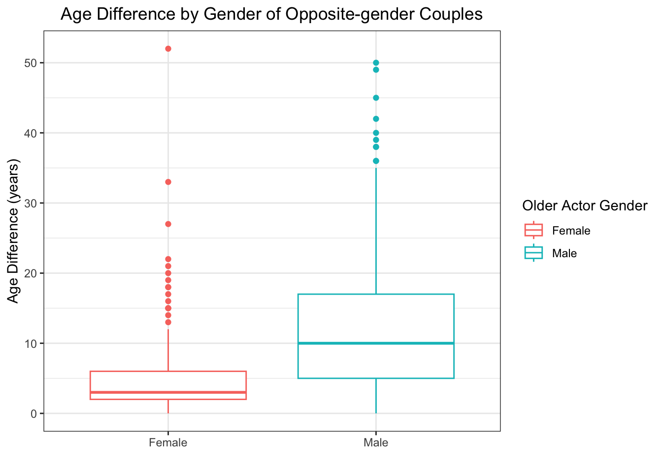
This is a better way to see the distribution of age gaps where either a male or female is the oldest in the relationship. We can see that on average, males are typically older than the females and the age gap is higher for older male-younger female relationships.
4. Do we see a greater age gap between same-gender or opposite-gender couples?
age_gaps3 %>% ggplot() + geom_boxplot(
  aes(
    x = gender,
    y = age_difference,
  color = gender))+
  theme_bw()+
  labs(
    x = "",
    y = "Age Difference (years)",
    title = "Age Gaps between Same/Opposite Gender Couples")+
  theme(
    plot.title = element_text(hjust = 0.5),
    legend.position = "none")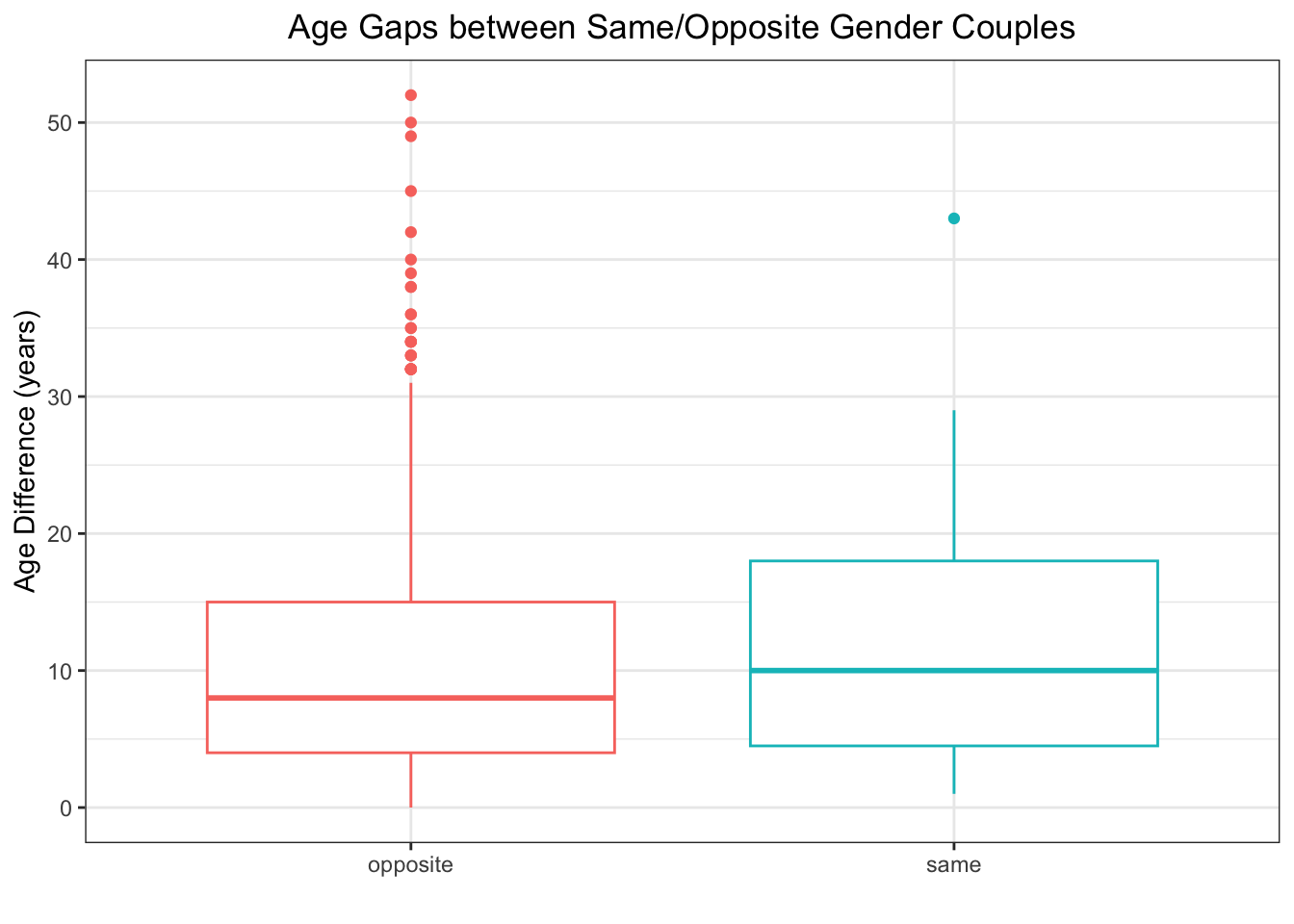
On average, there is a greater age gap in same gender couples, but it is important to note that there are only 23 entries for same-gender couples and 1132 entries for opposite gender couples. So this isn’t very informative.
5: How has the prevalance of same-gender relationships in movies changed over the years?
Same-gender prevalence in film
age_gaps3 %>% ggplot() + geom_point(
  aes(
    x = release_year,
    y = age_difference,
    color = gender,
    alpha = gender))+
  theme_bw()+
  scale_color_manual(values = c("dif" = "grey", "same" = "darkred")) +
  labs(
    x = "Release Year",
    y = "Age Difference (years)",
    title = "Prevalance of Same-gender Relationships in Film")+
  theme(
    plot.title = element_text(hjust = 0.5),
    legend.position  = "none")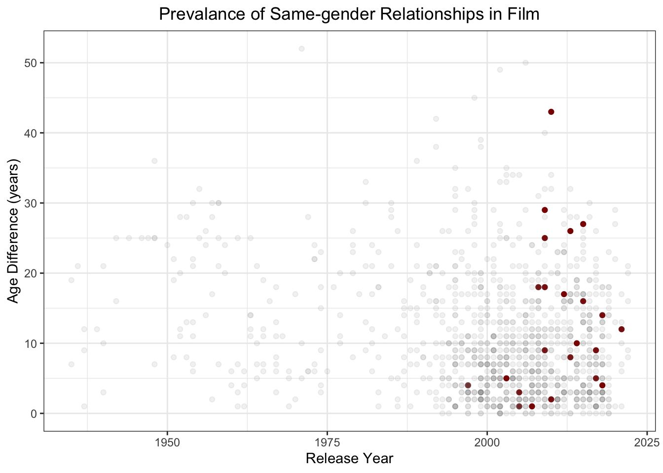
From our age_same data set, we can see that same-gender couples were documented starting in the year 1997 and that there are 23 recorded cases. We see a wide spread in age gap and that the prevalence of same-gender couples in the documented films increases starting after 1977.